Estimating fractal dimension of point datasetsCreated by Paul BourkeJuly 2018 Introduction The following documents a utility the implements a box counting estimate of fractal dimension for 3D point sampled datasets. The points are read as a simple text file, typically one 3D vertex per line, the x,y,z components separated by "white" space (most commonly spaces or tabs). The number of boxes N of size s are determined across a range of box sizes, the slope of the curve of log(N(s)) vs log(1/s) being the estimate of the fractal dimension. Command line usageUsage: pointboxcount [options] pointfilename Options: -bmin n Minimal box size (default: range/200) -bmax n Maximum box size (default: range/4) -dmin n n n Lower bounding box (default: auto) -dmax n n n Upper bounding box (default: auto) -bfact n Box size multiplicative factor (default: 1.5) -oset n Number of offsets used (default: 10) -skip n Skip n header lines (default: 0) -xy Enable projection onto the xy plane (default: off) -xz Enable projection onto the xz plane (default: off) -yz Enable projection onto the yz plane (default: off) -pov Save as Povray, mostly for debugging (default: false) -obj Save as OBJ, mostly for debugging (default: false) -v Verbose mode, default: offOptions When the points are read the bounding box of the data is determine and then used as the range on each orthogonal axes for the box counting search. There is no point searching outside this bounding box for points. The range of box sizes can be specified (-bmin,-bmax) otherwise it will be automatically chosen. This automatic choice is based upon the diagonal of the bounding box of the data, namely, a factor or 4 for the largest box and a factor 200 for the smallest box. This typically results in a range between one and two orders of magnitude. The progression of box sizes is determine by -bfact, a multiplicative factor. So if the smallest box size is S and the factor is 1.5, the sequence of box sizes will be S, 1.5*S, 1.5*1.5*S, 1.5*1.5*1.5*S ... and so on. Good estimates of box counting dimension requires that one finds the minimum box coverage for each box size. This is accomplished by randomly offsetting the origin for the boxes. The -mset option specifies the number of random offsets used per box size. In theory one should also vary the rotational axis for the boxes, for practical reasons this is problematic and not implemented here. Various output files can be generated to assist with checking and/or creating illustrative images, these include OBJ or POV files. Both contain axes, bounding box, the points themselves and the progression of boxes. The basis for the POVRay rendering might be the following: scene.pov and scene.ini. The images shown below were created with the POVRay output. OutputThe primary output is a text file containing the box size (s), the box count (N(s)), logarithm of the inverse of the box size and logarithm of the box count. An example is shown below.
A linear regression is performed and presented on the command line but users are encouraged to plot the points and ensure the linear portion of the curve is used. For example, very small box sizes and very large box sizes may result in spurious results. As an example, in the following an extreme range of box sizes is specified. The curve at the left (large box sizes) is where the box size is so large there is always only a count of 1, that is, the data fits within one box. The curve at the right is where the box size is so small that only one point is ever within a box, so the box count is just the number of points. 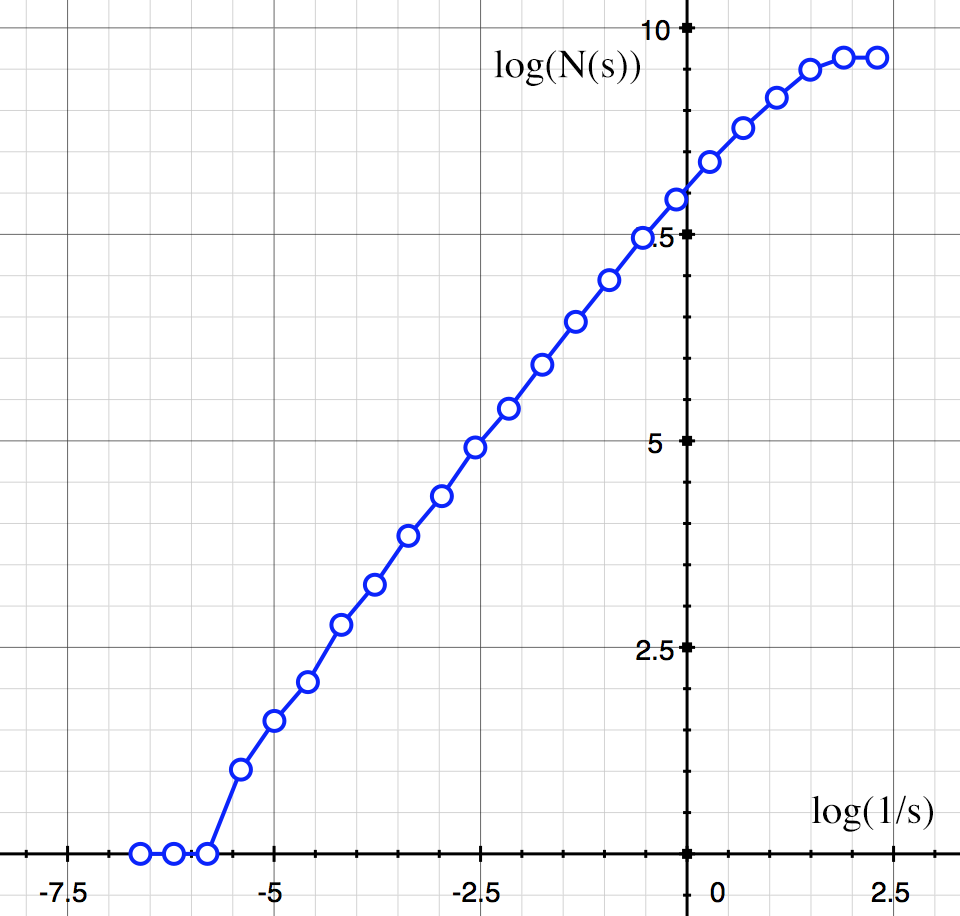
Some example datasets are illustrated below, mostly used during software testing. It should be noted that for various reasons one does not expect results identical to theoretical. These include the fact that many of these forms only have the theoretical dimension when iterated to infinity, some are continuous while these are point approximations and finally some are defined spatially to infinity whereas in the calculator here the area outside the bounding box is assumed empty. Example 1The triangular gasket, as shown below. 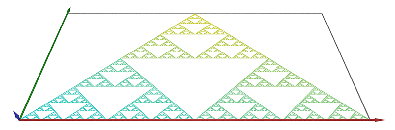
The theoretical value is log(8) / log(2) = 1.58. The log(N(s)) vs log(1/s) graph is shown below along with the slope estimate of 1.56. 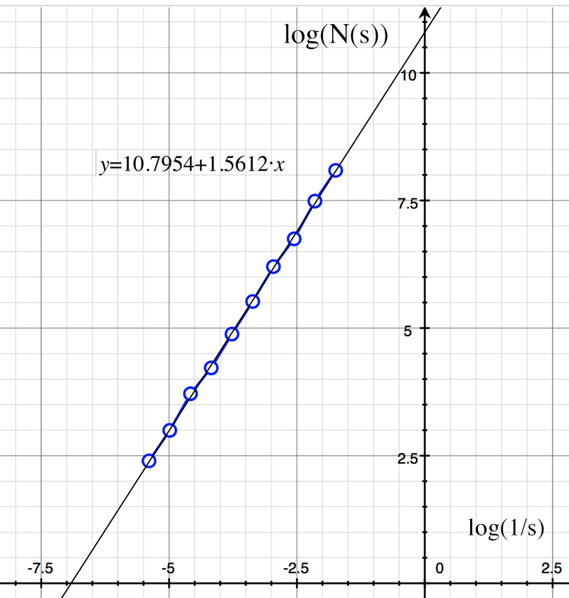
Example 2 Cantor dust embedded in 3D as shown below. 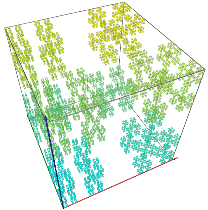
The theoretical value is log(8) / log(3) = 1.8928. The log(N(s)) vs log(1/s) graph is shown below along with the slope estimate of 1.86. 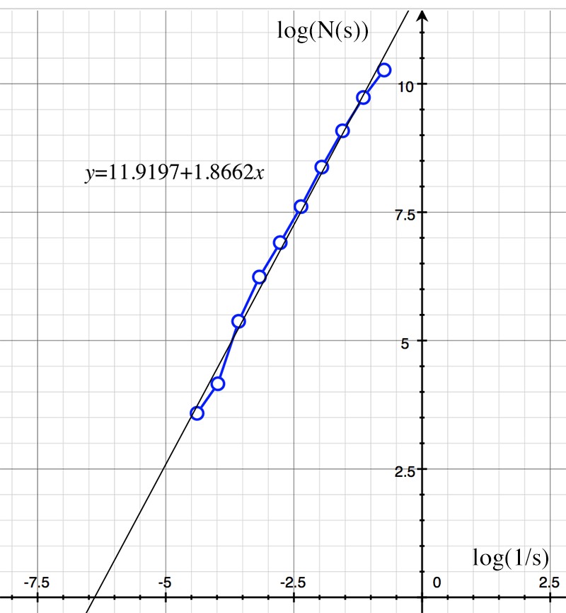
Example 3 A simple non fractal object, a line embedded in 2D. 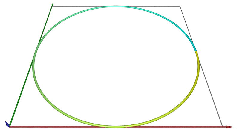
The theoretical value is 1. The log(N(s)) vs log(1/s) graph is shown below along with the slope estimate of 1.018. 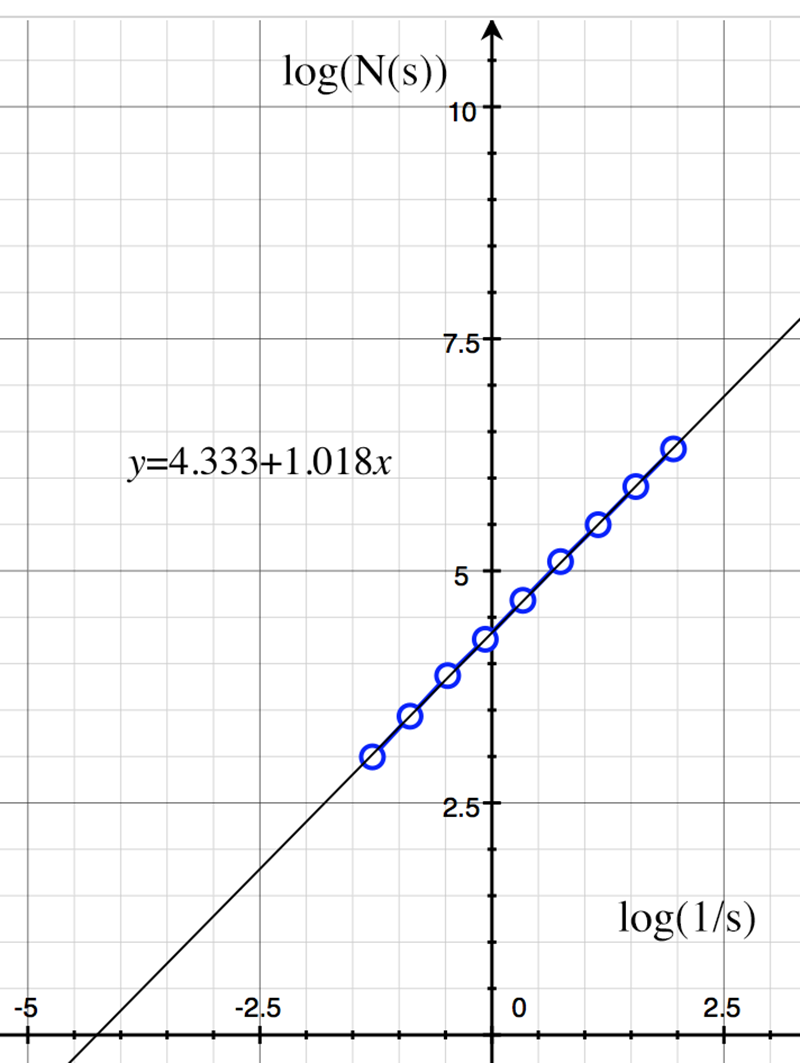
Example 4 The classic Von Koch Snowflake, as shown below. 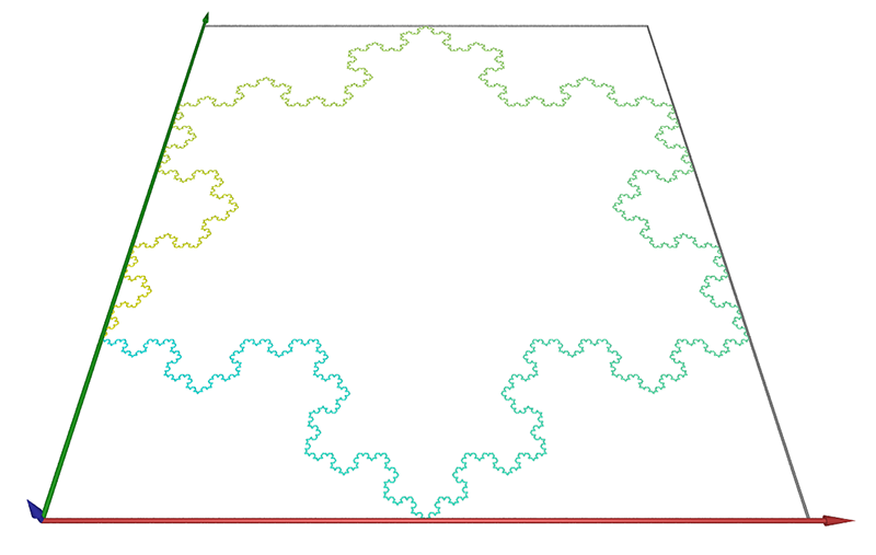
The theoretical value is log(4)/log(3) = 1.262. The log(N(s)) vs log(1/s) graph is shown below along with the slope estimate of 1.277. 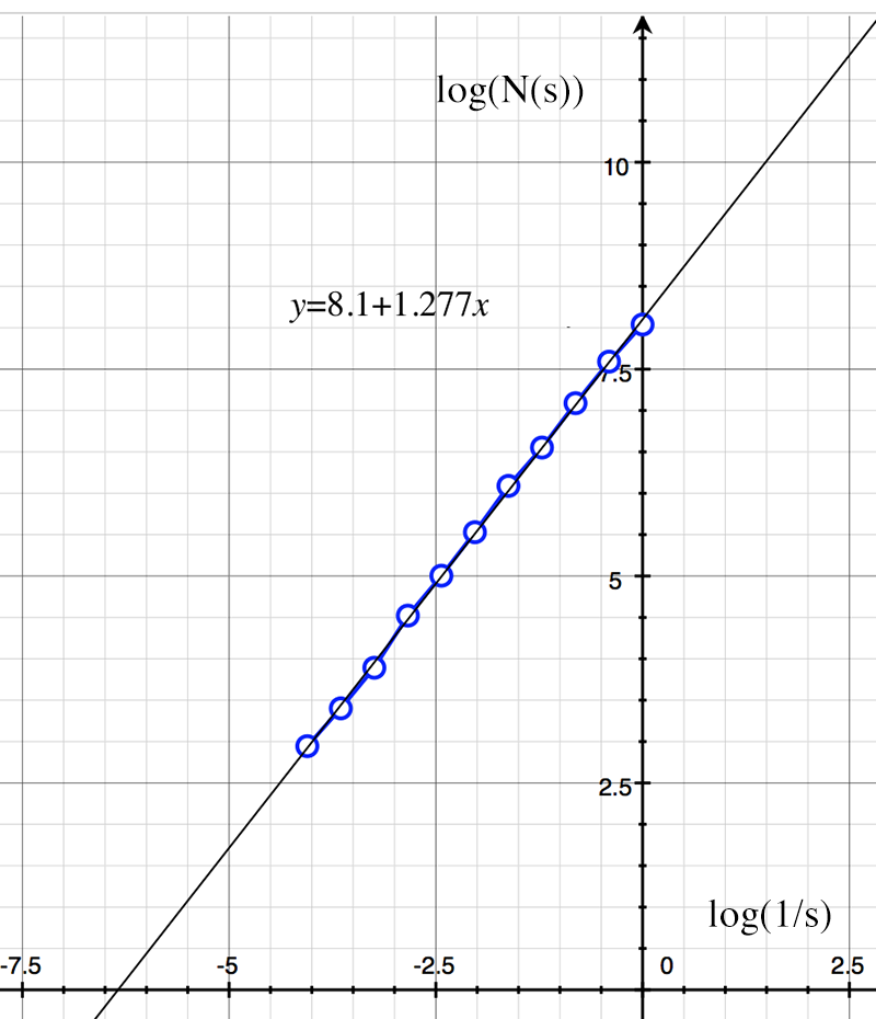
|