Logistic Equation and
Bifurcation Diagram

The standard form of the so called "logistic" function is given by

Where R is called the growth rate when the equation is being used to model population growth in an animal species say.

It was popularised by a review article written by Robert May in 1976 as an example of a very simple non-linear equation being able to produce very complex dynamics.

When used to create a series

This series behaves in one of the following ways depending on the value of R, the initial conditions don't matter (within reason).

• Extinction (Uninteresting fixed point)
  If the growth rate R is less than 1 the system "dies", A_n -> 0.

• Fixed Point
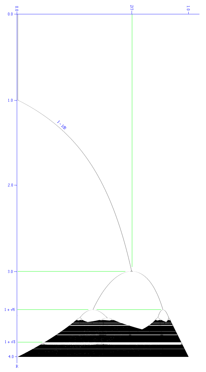
  The series tends to a single value. How it reaches this value is not important but generally it oscillates about the fixed point but unlike a mass spring system, the series generally tends to rapidly approach fixed points. In the bifurcation diagram below the system can be seen to tend to fixed points for 1 < R < 3.

• Periodic
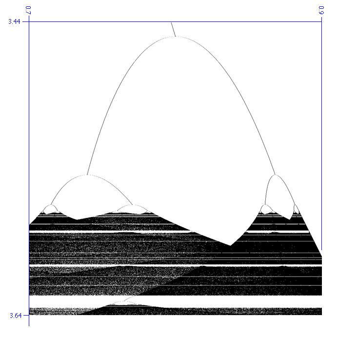
  The series jumps between two or more discrete states. In the bifurcation diagram below it can be seen that the system alternates between 2 states after R = 3. After about 3.44948 (1 + sqrt(6)) the system alternates between 4 states. Notice the system jumps between these states, it does not pass through intermediary values. The number of states steadily increases in a process called period doubling as R increases. For example at 3.5441 until 3.5644 there are 8 states. Between 3.5644 and 3.5688 there are 16 states.

• Chaotic
  In this state the system can evaluate to any position at all with no apparent order. In the bifurcation diagram below, the system undergoes increasingly frequent period doubling until it enters the chaotic regime at about 3.56994. Below R = 4 the states are bound between (0,1), above 4 the system can evaluate to (0,infinity).
  Amongst this chaos a 3 period surprisingly appears between about 3.8284 (1 + sqrt(8)) < R < 3.8415.

The following is known as a bifurcation diagram, it shows the values the system (series) evaluates to for different values or R. In practice this diagram is generated by choosing a random initial value in the range (0,1) and evaluating the first N terms of the series for a suitably large value of N (say 1000). At this point the system is considered to have settled down and the next M terms of the series are plotted, again for a suitable large M (say 10,000).

Zooming in to show the period doubling more clearly.

A particularly interesting feature of period doubling is the ratio between consecutive period doubling intervals, it is a constant known as the Feigenbaum number.