samila mappingsWritten by Paul BourkeAugust 2023 Brought to my attention by Patrick Kubisch First known implementation by Sepand Haghighi and Sadra Sabouri.
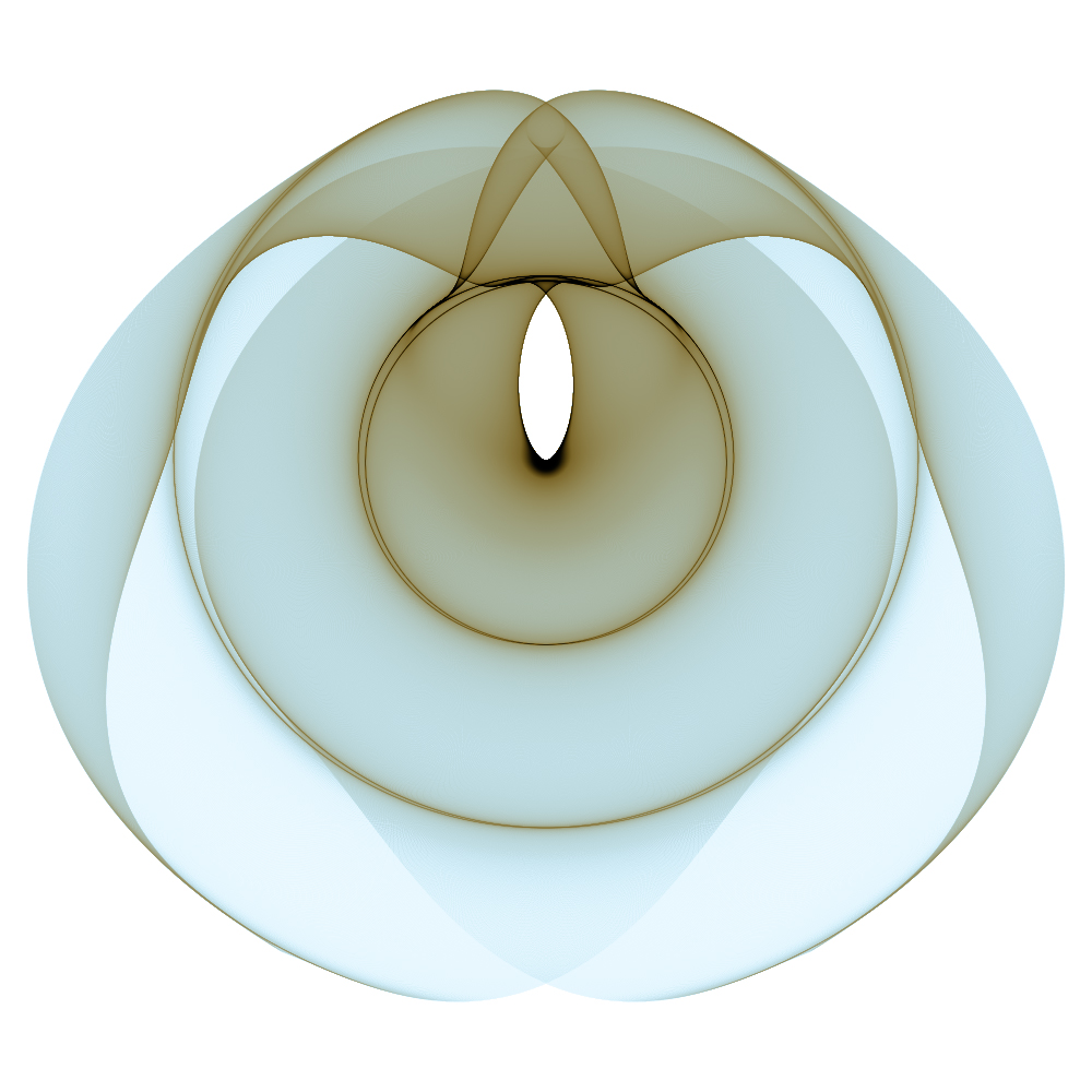
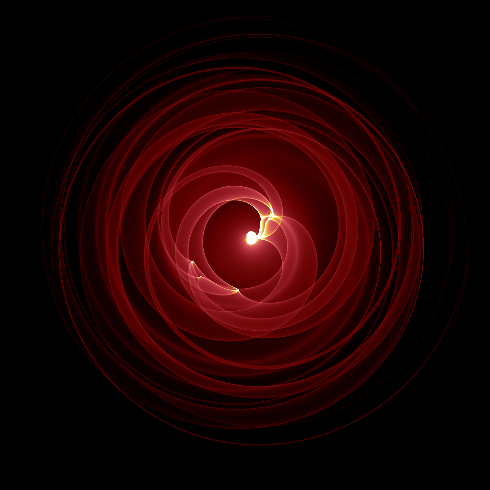
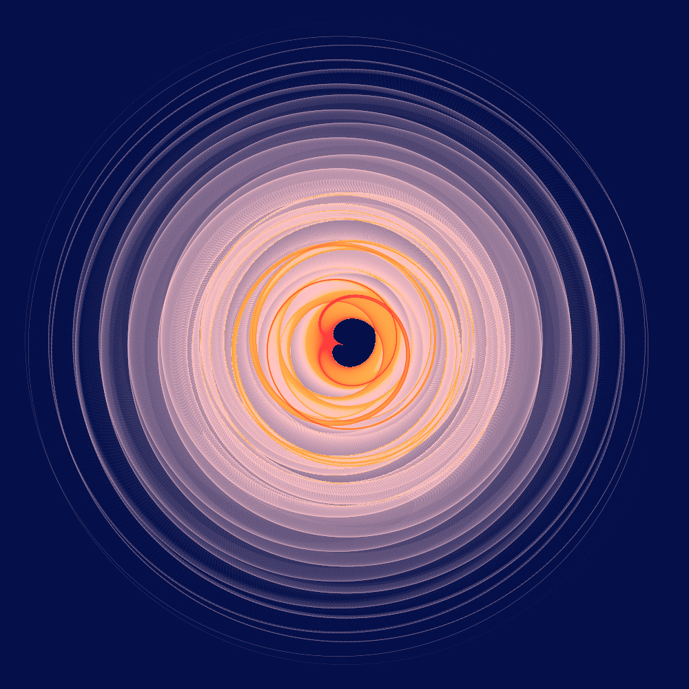
The following are example of so called "samila" mappings. While they are listed here in the fractals/chaos section they are not chaotic attractors, although they do share a visual similarity with many attractors. 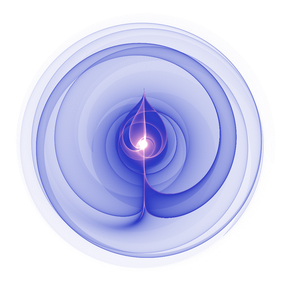
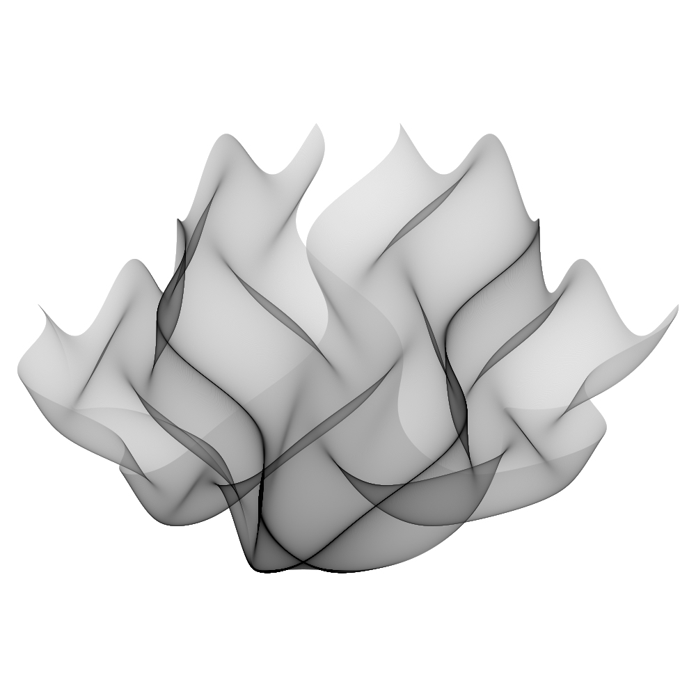
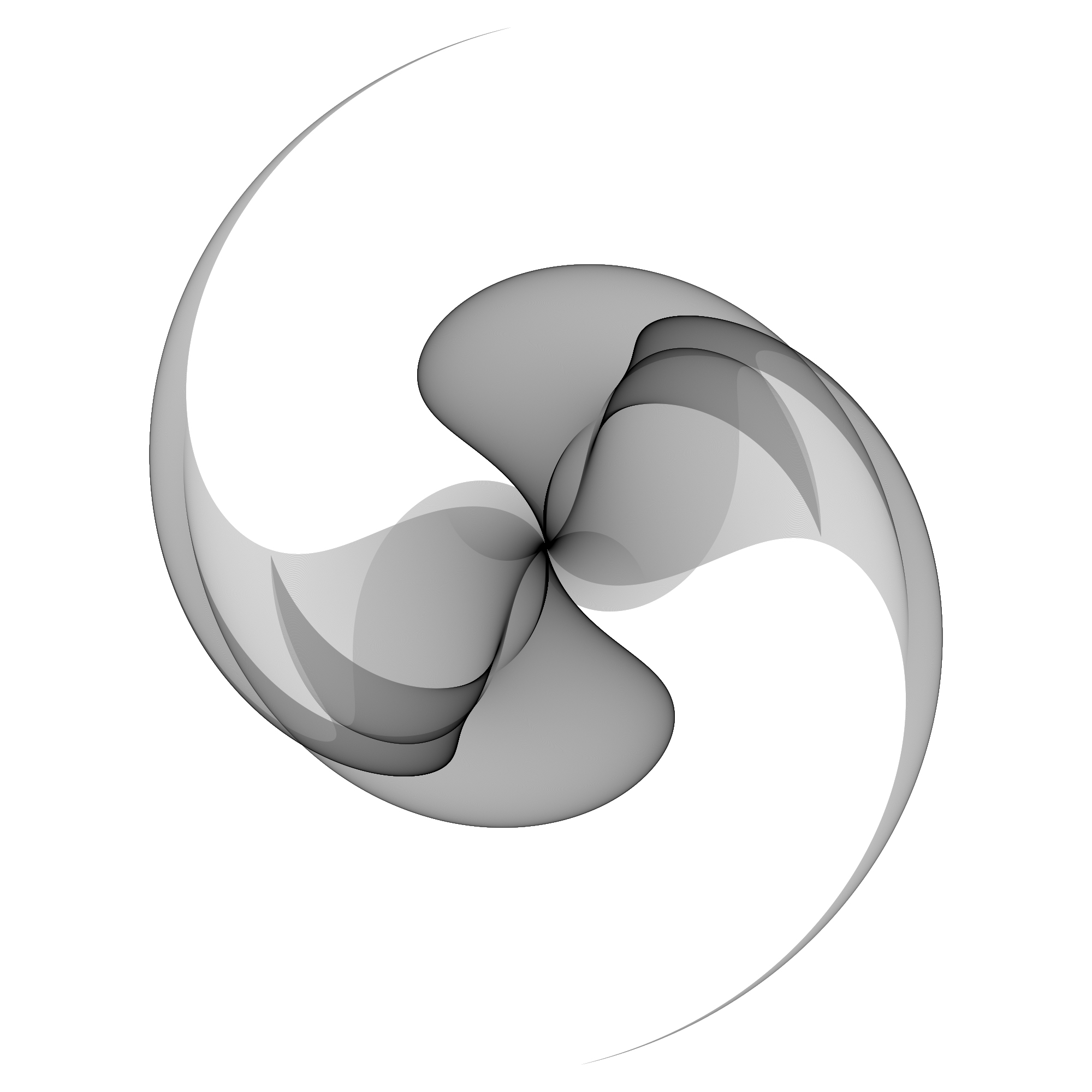
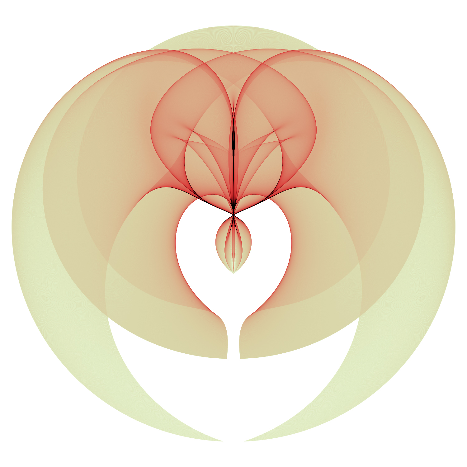
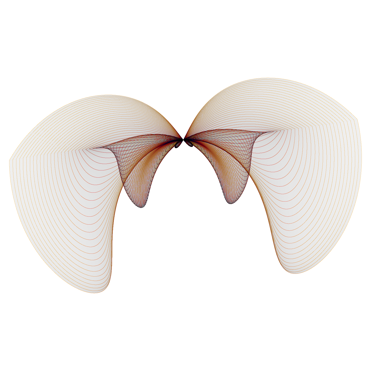
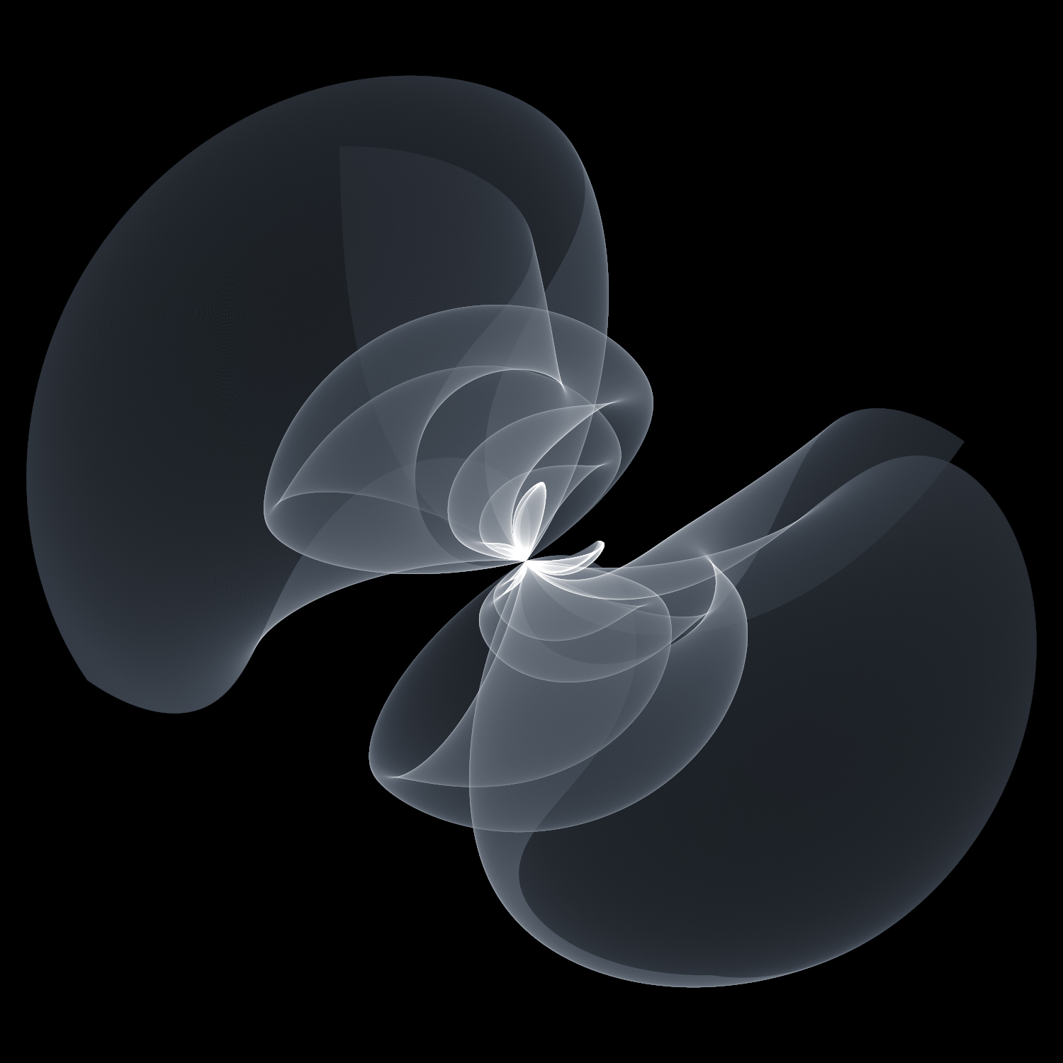
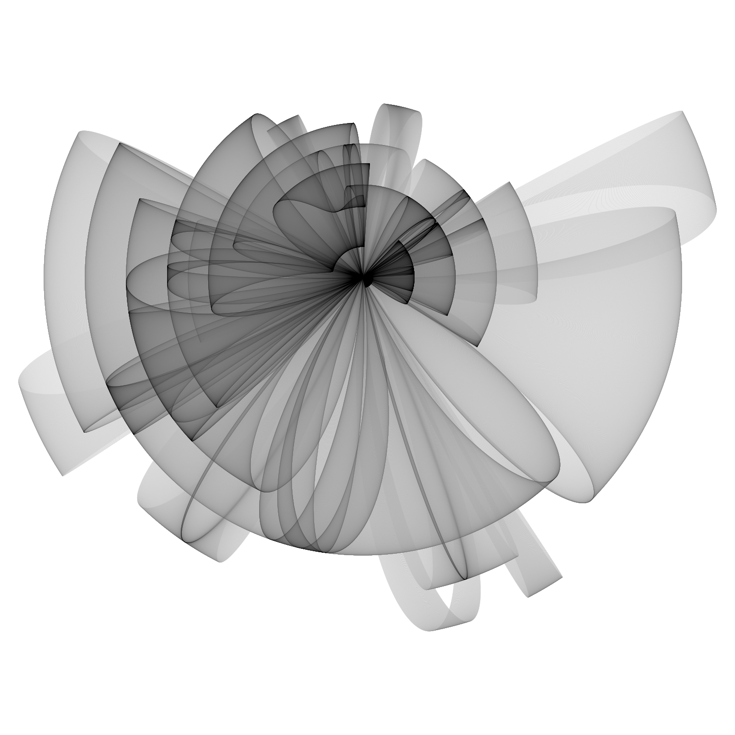
They are a mapping from a rectangular region on a plane to another region on the plane. The intensity/colour in the images found here indicates the density of the remapped points in the destination region given a uniform sampling density of the source region. 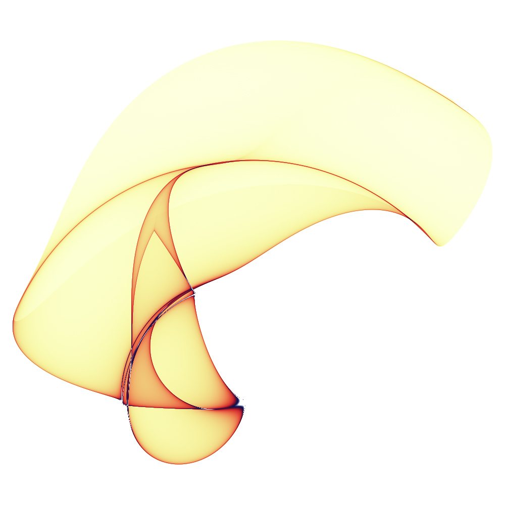
The transformations involve two functions of x and y, mapped to positions x' and y', that is: 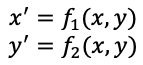
The mapping may be direct or interpreted as polar coordinates, for example: 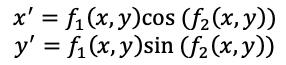
In the original publication the functions f1(x,y) and f2(x,y) are as follows. But there is a small infinity of possible functions that could be used. The implementation here has a collection of 50 different functions that can be used for either f1 or f2. 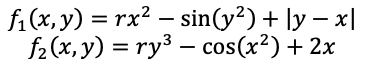
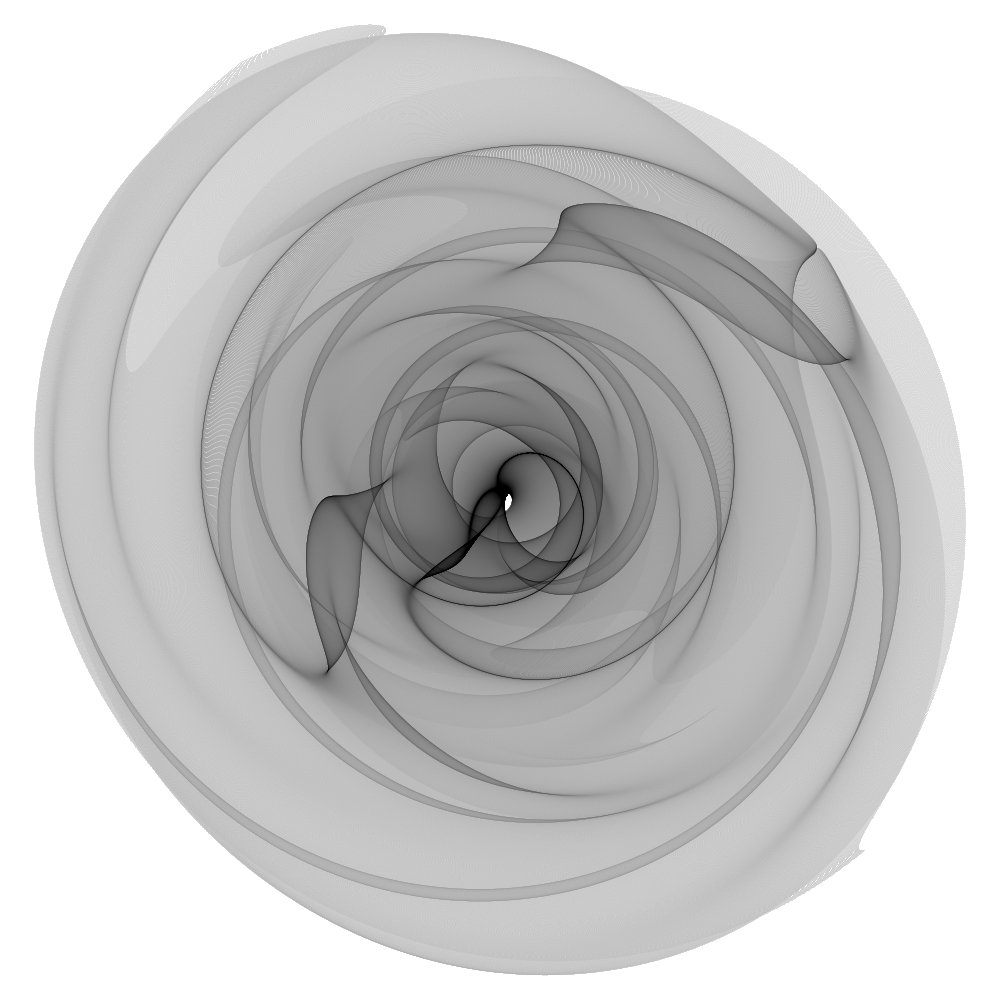
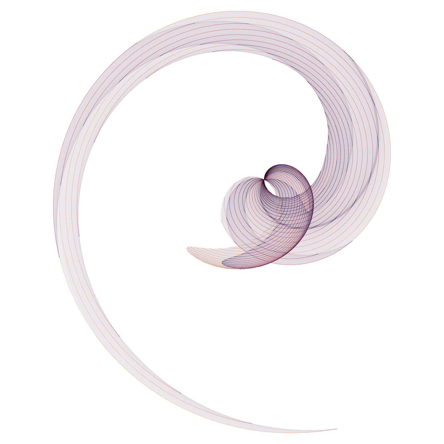
Where "r" is a random number in the range of -1 to 1. The resulting mappings are given below, for a particular random value r. The left is the direct mapping, on the right is the polar mappings. All other images on this page use the polar mapping.
Different images can be created by changing the random variable, as such, to be able to recreate a particular image the random number seed needs to be recorded along with the two functions used. It should be noted that the appearance of the final image doesn't always change radically with the random variable. 
Since the mappings often involve trigonometry functions, the source region range is usually taken as from -π to π, but this is not a requirement. 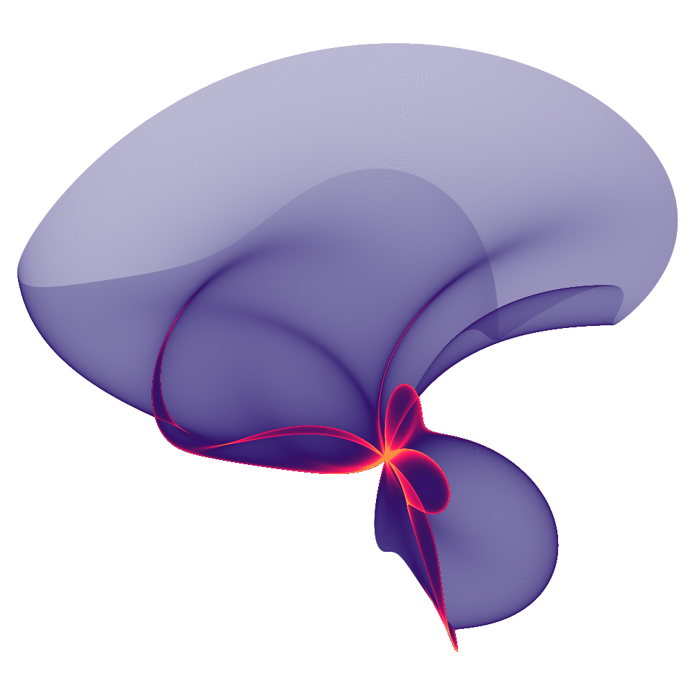
The colouring used in this document is not part of the generation process. The implementation generates a 16 bit greyscale raw image. This can be opened in PhotoShop (and others) and a colour gradient designed and applied to the greyscale image. 
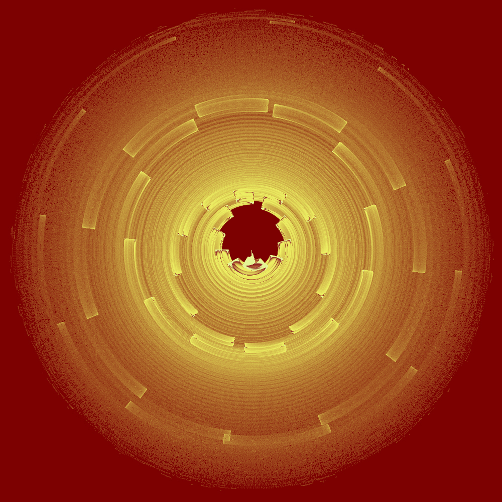
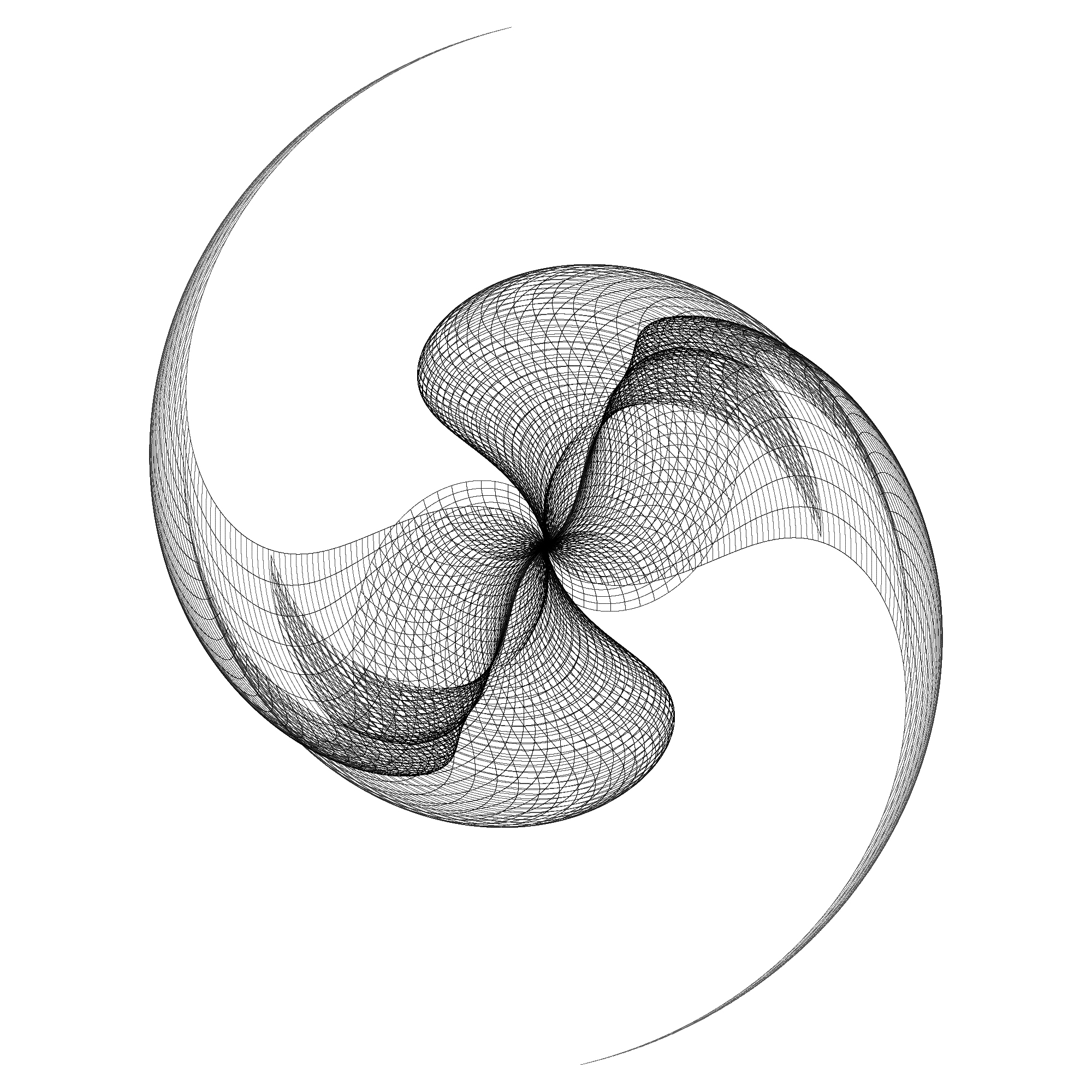
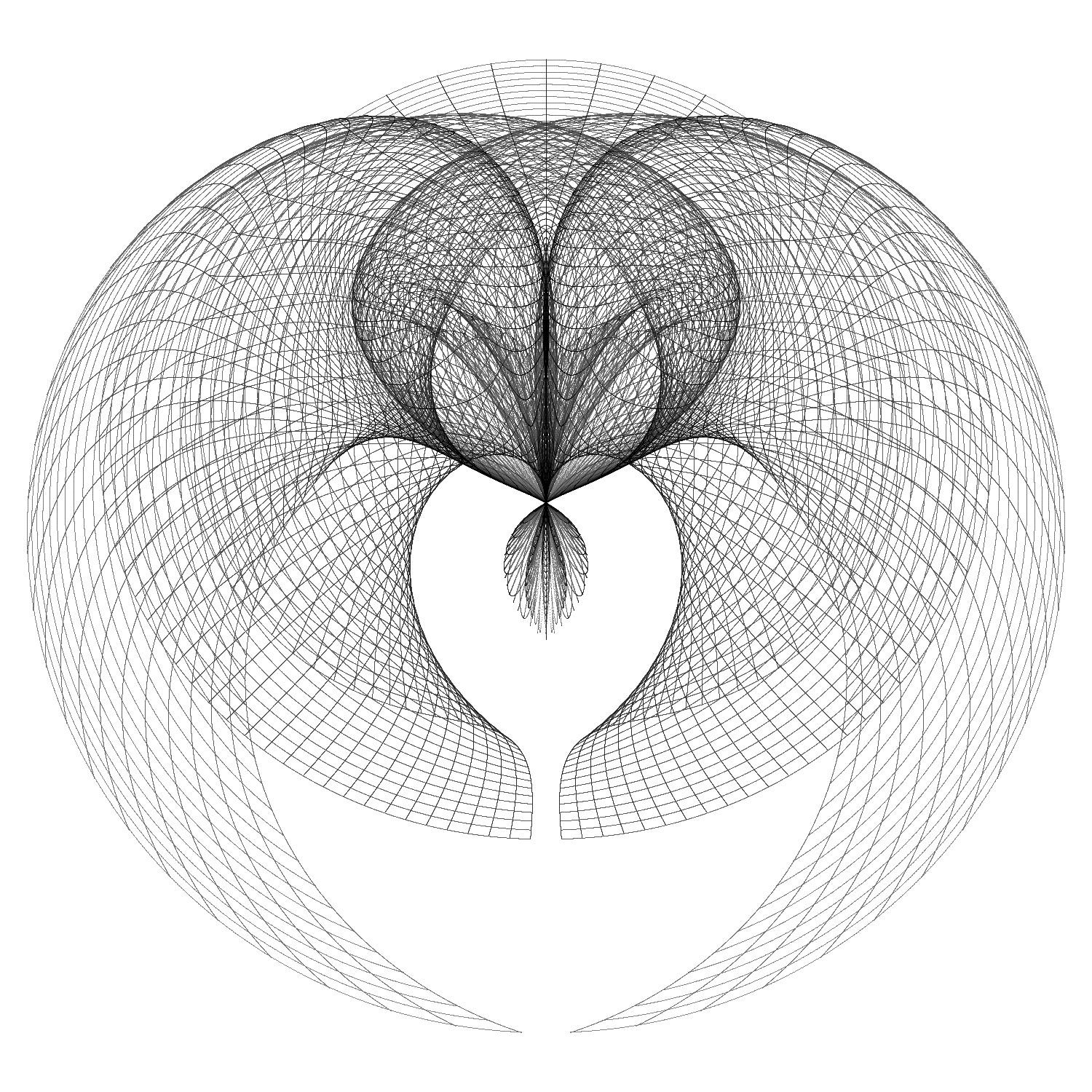
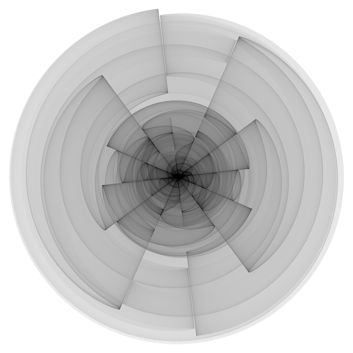
As a variation, instead of sampling the source region uniformly, one can sample very densly in one axis and less in the other. This illustrates very clearly how a source grid would be transformed. 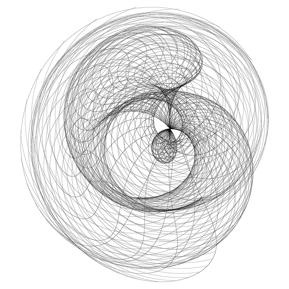
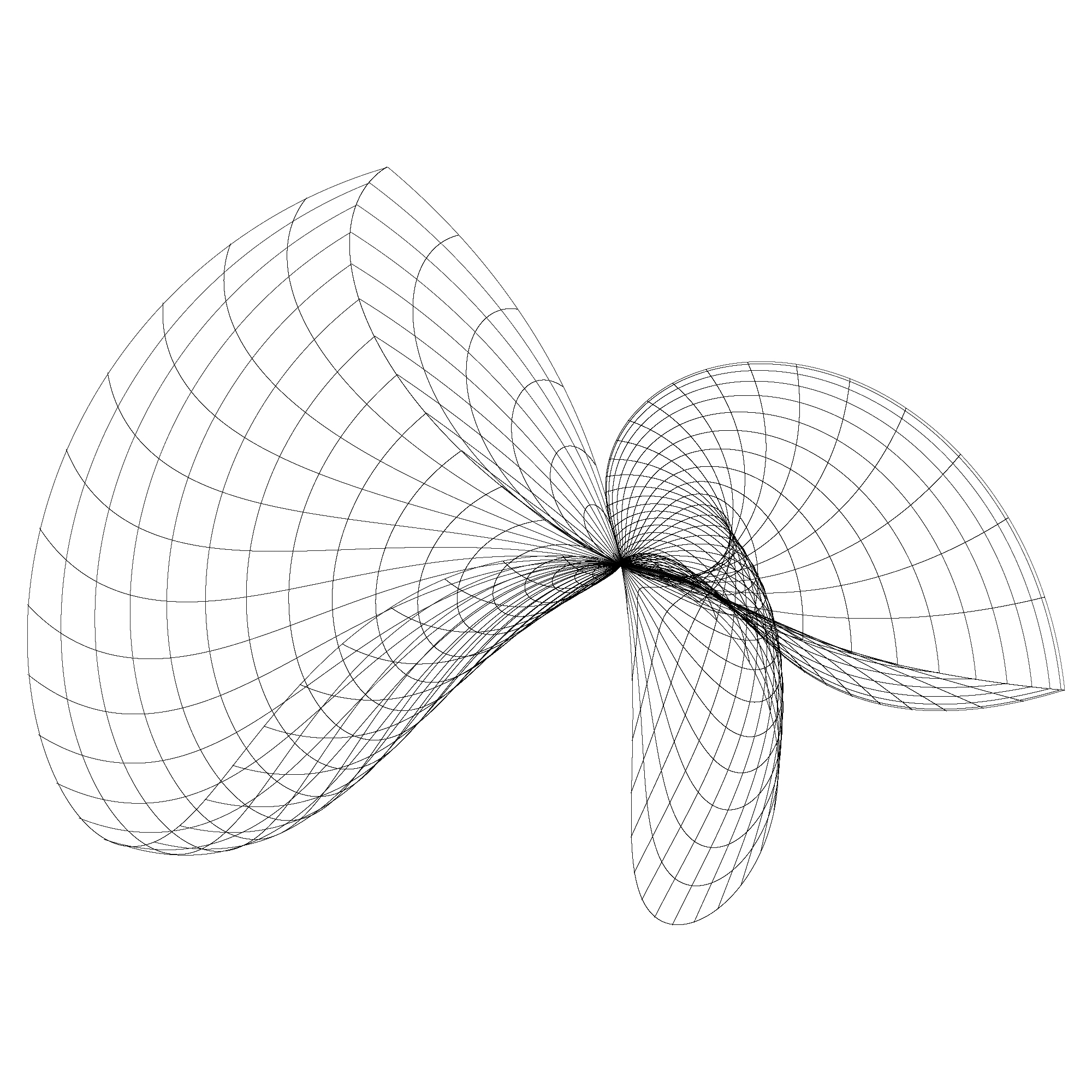
Just like some attractors (Clifford attractors) these often look as if they are projections of a 3D shape. In reality they are purely 2D functions. 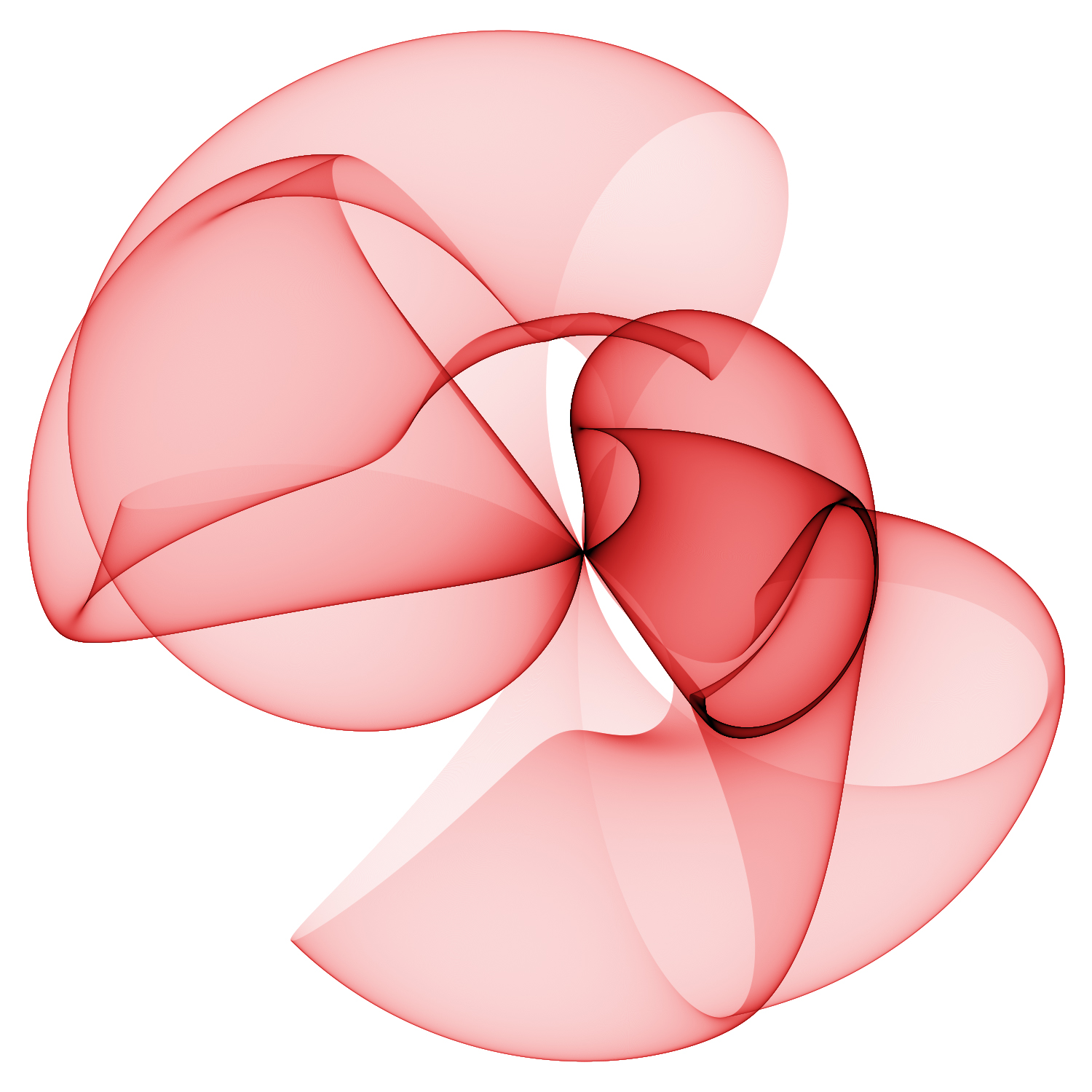
|