This document is the user manual for a program on the Macintosh for exploring 4 dimensional geometry. Here we will introduce the concepts of 4D geometry, describe the use of the application, and present some examples. Introduction
Hyperdimensional objects
The geometry of familiar objects in higher dimensions is well established mathematically but is generally outside our everyday experience. A mathematical approach will not be attempted here but rather the intuitive description of 4D geometric objects. Generation by intuition
The creation of 4D geometric objects by intuition relies on being able to
determine an progressive description of the equivalent object in 3D and how it
was created from its 2D equivalent. If we "know" how the 3D object is created
from 2D and maybe how the 2D object was created from 1D then the rules can be
applied to the 3D object to form the 4D equivalent.
A one dimensional cube is a line segment. To create a 2D cube, a square. we "extrude" the line (1D cube) along the newly introduced axis. To form the 3D cube we again extrude the square (2D cube) along the newly introduced axis. So the general technique for generating a n+1 dimensional cube is take the n dimensional cube and extrude it along the new n+1 dimension. 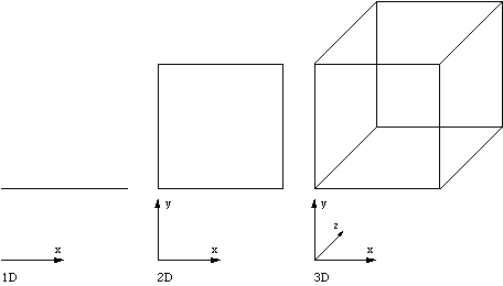 Tetrahedron
1D tetrahedron is a line. 2D tetrahedron is an equilateral triangle. The n+1 dimension tetrahedron is created by taking the midpoint of the n dimensional tetrahedron and pulling it into the n+1 dimension. 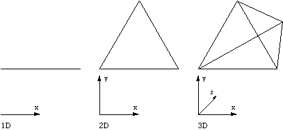 Octahedron
1D octahedron is a line. 2D octahedron is a square. To form a n+1 dimensional octahedron take the midpoint of the n dimensional octahedron and pull it along the positive and negative axis of the n+1 dimension. 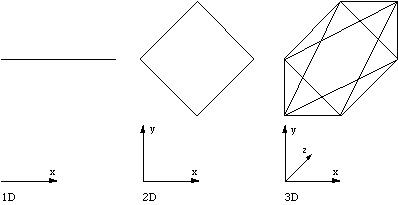 Pyramid
To create a n+1 dimensional square based pyramid take the n dimensional cube and pull the midpoint into the n+1 dimension. 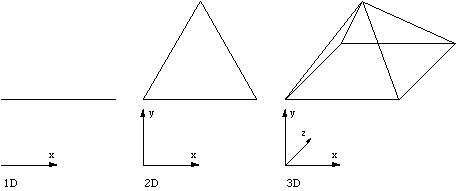 Prism
A n+1 dimensional prism is the n dimensional cube with two opposite midpoints pulled into the n+1 dimension. 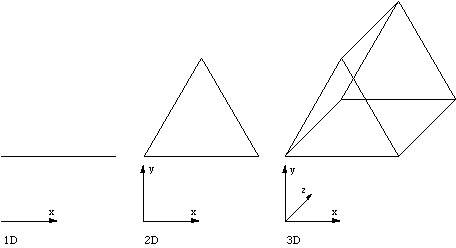 Display techniques
The main visualization problem associated with 3D modelling is how to represent a 3D scene on a medium with one fewer dimensions, ie: a computer screen or piece of paper. This problem is made much more difficult for HyperSpace since now we need to represent 4D objects on a medium with two fewer dimensions. HyperSpace employs four fundamental techniques to solve this problem, they are discussed below. Parallel Projections
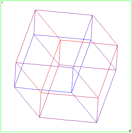
In order to visualize 3D objects on a 2D medium it is common to simply ignore one coordinate. For example: ignore the z coordinate and draw the x and y coordinates. Such a technique gives what are called parallel projections and isometric projections of 3D objects. This technique can be used to represent 4D objects on a 2D medium, however in this case we have to ignore two coordinates. For example: ignore the w and y coordinates and draw only the x and z coordinates. This is what the xy projection menu item in the view menu does. One should be very wary about trying to visualize the geometry of a 4D object by this technique. It is analogous to trying to visualize the geometry of a 3D cube by projections of it onto a line. HyperCube examples
 Elevations and plans
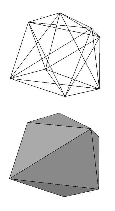
Another technique employed to represent 3D objects on a 2D medium is to project the object onto each coordinate plane, xy, xz, and yz. 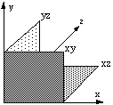
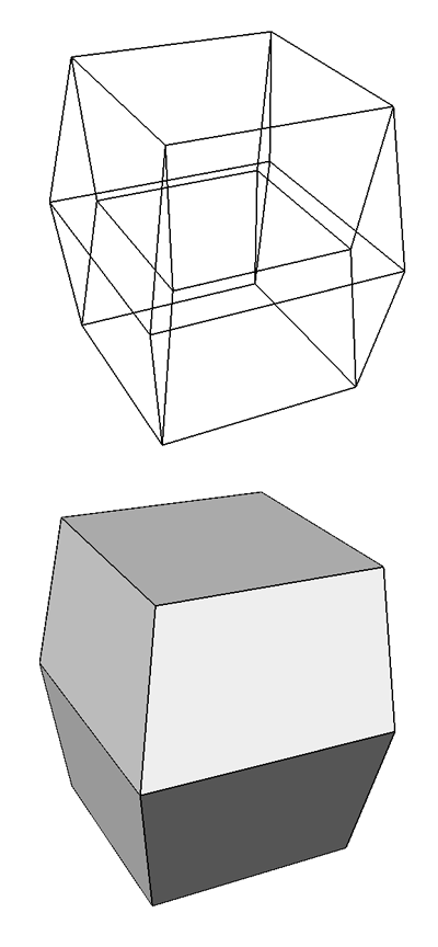
This gives the common top/bottom (plan), front/back (elevation) and left/right views of a 3D object. For example a simple 3D structure is shown below with the projections onto the three coordinate planes. 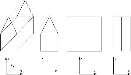
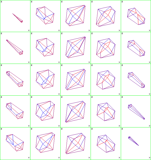
This technique can be used for 4D objects except that there are six 2D projection planes, namely wx, wy, wz, xy, xz, and yz. Each of these can be displayed in the six views window shown below 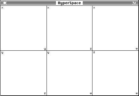
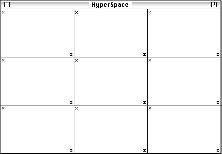
Note that the axes labels are placed in the top-left and bottom-right of each view portion. The three view portions in the top left corner correspond to the top, front, and side views in 3D. For an unrotated HyperCube the six axis views are quite boring, they are all squares. The following shows the 6 axis views if the HyperCube is rotated on all planes.  Slices
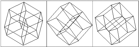
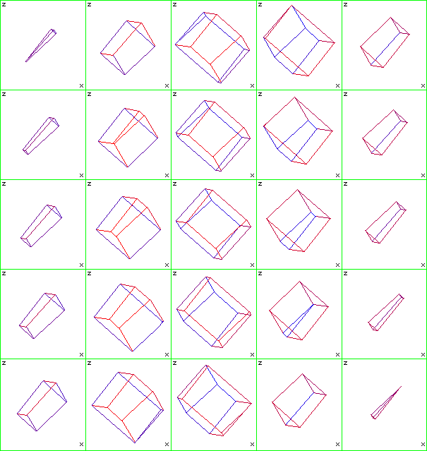
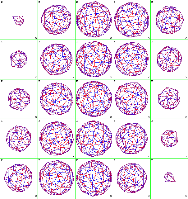
The third technique used to represent 3D objects on a 2D medium is to contour the object, effectively cutting slices along one coordinate axis. It is usual in 3D to take the contours along the z axis but any axis will do. An arbitrary slicing plane may also be used or alternatively the contours can always be with respect to one axis and the object rotated in order to obtain arbitrary slicing planes. This process essentially removes one dimension, so slicing a 3D object results in a series of 2D curves. the contour lines. To contour 4D objects we will choose to always slice along the w axis. Removing one dimension from 4D objects results in a series of 3D objects which can be projected by any of the classical techniques. The window for 9 slices is shown below
The window for different numbers of slices simply partitions the window into smaller view portions. The axes labels are shown, the w axes is the one along which the slices are taken, the y axes is ignored (projected onto the x-z plane). Nine slices of the HyperCube are shown below. It doesn't seem that difficult to imagine each of the solids below.....the problem comes when you need to stack them up together in the 4th dimension. 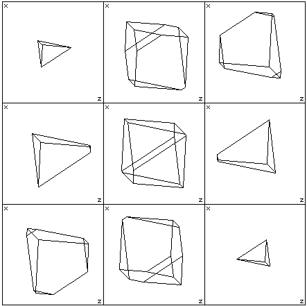 Depth Cue
The last technique which can be used in conjunction the others is to shade the edges according to the value of one coordinate. In the HyperSpace application, points with a large y coordinate may be shaded red, points with a small y may be shaded blue and all points in between are coloured with the appropriate intermediate hue. 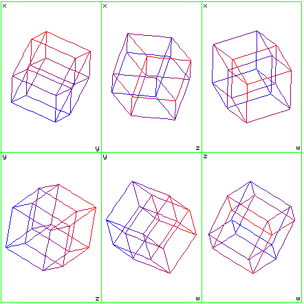
Rotating the object
When viewing an object using a computer aided design package there are two operations which can be useful. They are: rotate the camera about the object or rotate the object about its centre. There are subtle differences between the two approaches, the HyperSpace application implements rotation of object about any one of the coordinate axis. Considering the situation in 3D, there are three axes, x,y, and z about which an object can be rotated. Alternatively there can be considered to be three planes through which an object may be rotated. The two descriptions are identical, the only difference is in how they are described. So, for example, rotation about the x axis is the same as rotation in the y-z plane, rotation about the y axis is rotation in the x-z plane and rotation about the z axis is rotation in the x-y plane. The rotation plane is the terminology used here. In 4D there are six planes though which an object can be rotated. The amount of rotation in each plane is specified with the rotate controls window shown below. Each of the six sliders ranges from -180 degrees at the top to 180 degrees at the bottom. By clicking on the arrows the angle varies by one degree intervals, by clicking in the grey region the angle varies in 10 degree steps. If the slider reaches the bottom of the scale it will wrap around to the top and similarly when the slider reaches the top it will wrap around to the bottom, ie: -190 degree rotation = 180 degree rotation. With dimension set to 3 the first three sliders are disabled. 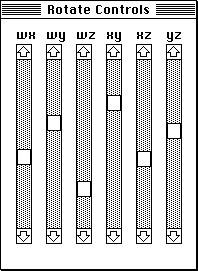
Reading models from a file
It is possible to use HyperSpace to view other 4 dimensional objects. To do this a specially formatted text file must be created describing the geometry. This file is opened with the read menu item in the file menu. The format will be described below but it should be stressed that the format must be closely adhered to if HyperSpace is to correctly read the object geometry. The text file consists of three sections, they are: the vertex description, the edge description, and finally the face description. Each section starts with the number of elements in that section, for example, the vertex section starts with the number of vertices that will follow, the edge section starts with the number of edges to follow, similarly for the faces.
Vertices: Each vertex appears on a line by itself and consists of four floating point numbers representing the w,x,y,z coordinates. Edges: Each line of the edge description contains two numbers representing the vertex numbers of the endpoints of the edge. Faces: Each line of the face description consists of five numbers. The first is the number of vertices in the face, it may be either 3 or 4. The remaining numbers are the vertex numbers making up the face. All four vertex numbers must be specified even if they are not used, the unused vertex number could be 0, it will be ignored in any case.
The vertices and edges must be present for any object description but the faces information is optional. If the faces are not specified then the number of faces must be set to 0. Note however that without faces the slicing method of visualization will not work. This format is the one generated when the save menu item is used in the file menu. An example of a correctly formatted file is shown below
5
-1 -1 -1 1
-1 1 1 1
-1 1 -1 -1
-1 -1 1 -1
1 0 0 0
10
0 1
0 2
0 3
1 2
1 3
2 3
4 0
4 1
4 2
4 3
10
3 0 1 2 0
3 0 1 3 0
3 0 2 3 0
3 1 2 3 0
3 4 0 1 0
3 4 1 2 0
3 4 1 3 0
3 4 0 2 0
3 4 0 3 0
This object contains 5 vertices, 10 edges, and 10 faces. Note from the edge list that the vertex numbers start from 0 not 1, so the vertex numbers in the edge and face list range from 0 to 4 not from 1 to 5. The face list consists of only 3 point faces, the fourth column must be present but it is only considered for 4 point faces. While all the numbers above are integers floating point numbers are equally valid. The separators between each number can be any "white" character, most commonly spaces or tabs would be used. This makes it possible to create these files with basic programs, spreadsheets, word processors, etc. References
Experiments in 4 Dimensions, Heiserman, David L., TAB Books Inc Regular Polytypes, Coxeter, H.S.M., MacMillam Company Introduction to Geometry, Coxeter, H.S.M., John Wiley & Sons Inc 4 Dimensional Space, Eckhart, L., Indiana University Press
Regular Polytopes (Platonic solids) in 4DWritten by Paul BourkeJune 1997 Update November 2003
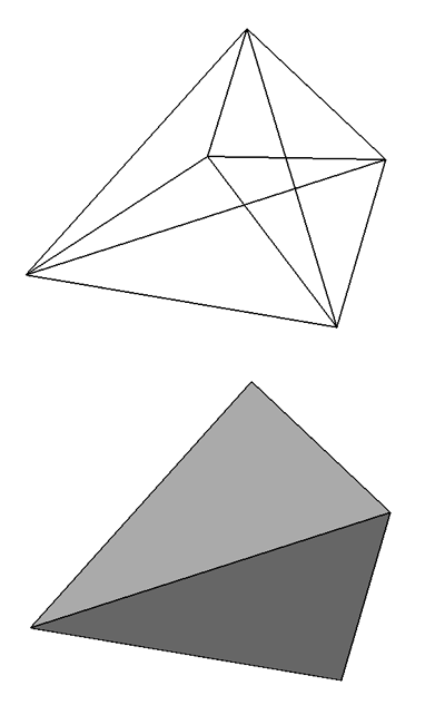
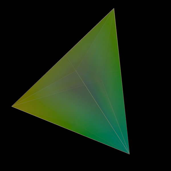
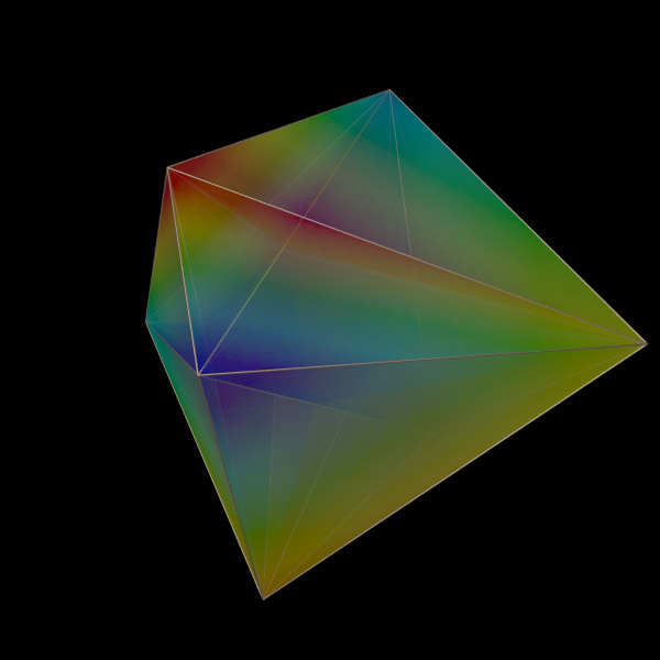
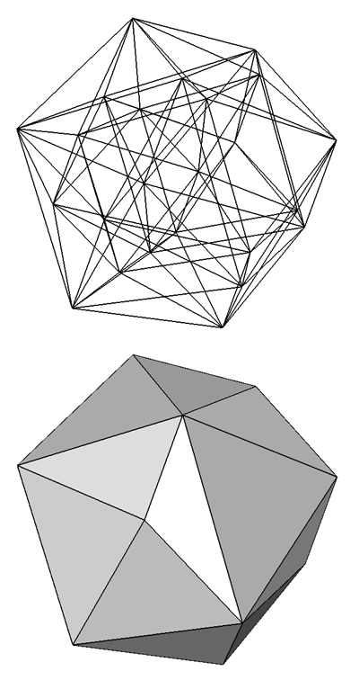
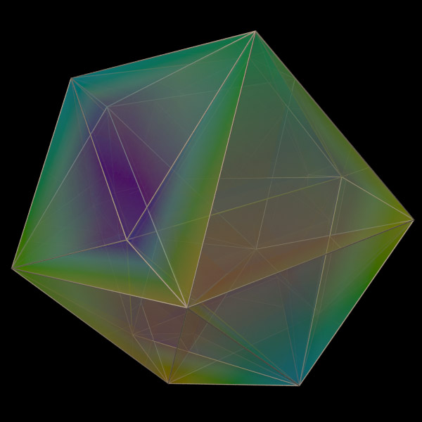
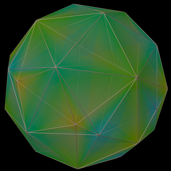
Regular polytopes or platonic solids are convex solids (closed) where all the building blocks (vertices, edges, faces, hyperfaces) have the same characteristics. That is, vertices have the same number of neighbours, edges are all the same length, polygons are all the same shape and area, and hyperfaces have the same volume. In 2 dimensions there an infinity of regular polytopes. For example, a circle can be approximated by polygons with 2 edges (line), 3 edges (triangle), 4 edges (square), 5 edges, 6 edges ..... indeed any number of edges. In 2 dimensions, every regular polytope is its own dual. In 3 dimensions there are just 5, these are typically known as the platonic solids. In 3 dimensions, the tetrahedron is self-dual. The dual of the cube is the octahedron. And the dual of the dodecahedron is the icosahedron. Regular polytopes in 4 DimensionsIn 4 dimensions there are 6 regular polytopes, this is the highest number that exist in any dimension greater than 2. They are listed and described in order of increasing cell numbers below. Each regular polytope is supplied as data in at least two versions, the first is a simple ASCII format listing vertices, edges, and faces. The second is as an OFF file ready for GeomView. Simplex
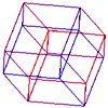
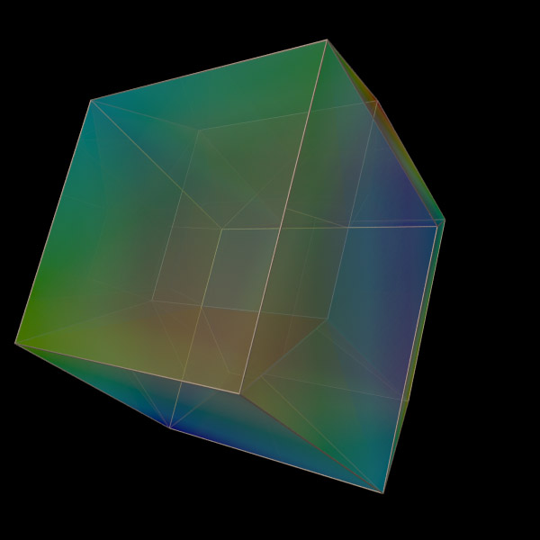
Hypercube
Cross Polytope
24 cell
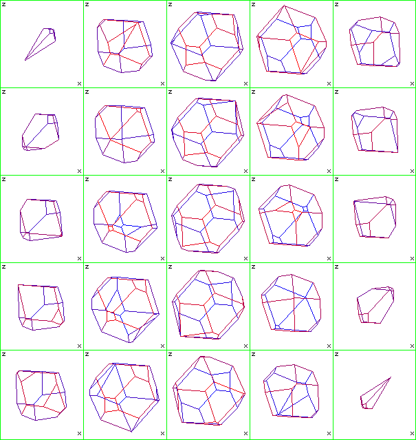
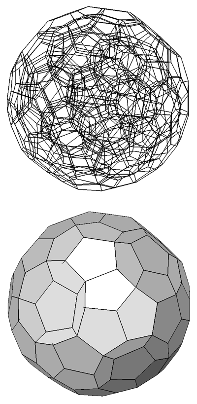
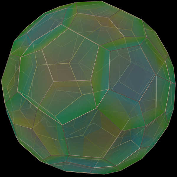
120 Cell
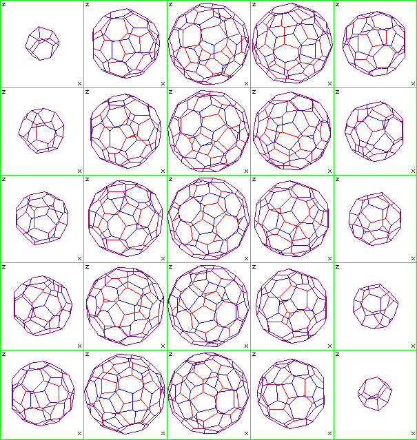
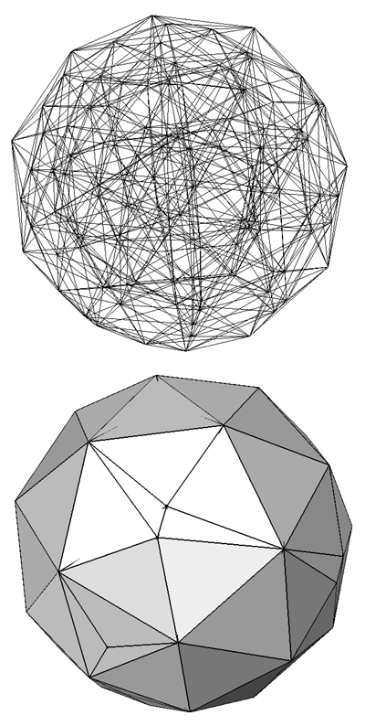
600 Cell
Higher Dimensions In higher dimensions (5, 6, 7 ....) there are only 3 regular polytopes in any particular dimensions! These 3 regular polytopes are the equivalent of the tetrahedron, cube, and octahedron in 3 dimensions, they are normally called the n-simplex, n-cube, and n-crosspolytope respectively where n stands for the dimension. n-simplex
n-cube
n-crosspolytope
Dual
Self-dual
Polyhedral formula
Vertex/Face ASCII format
Experiments in 4 Dimensions. Heiserman, David L. TAB Books Inc Introduction to Geometry. Coxeter, H.S.M. John Wiley & Sons Inc
4 Dimensional Space
Eckhart, L.
4D objects in VEF formatSourced mostly from Satoshi Yamaguchi and Gordon KindlmannCompiled by Paul Bourke |