Spherical HarmonicsWritten by Paul BourkeFebruary 1990
MSWindows interactive viewer:
SHDEmo.exe.gz contributed by Wolfgang Wester
Contribution by Georg Duemlein: pythonSOP
 Formulation
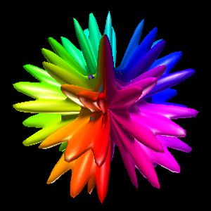
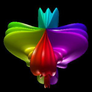
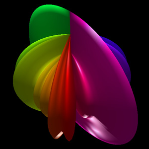
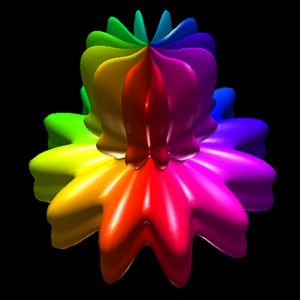
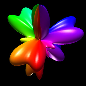
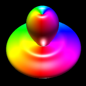
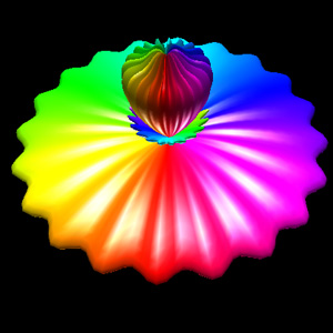
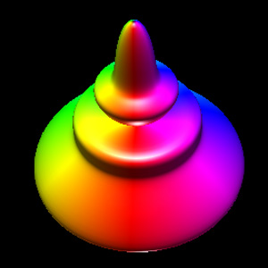
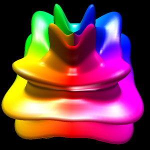
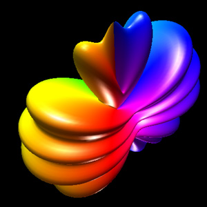
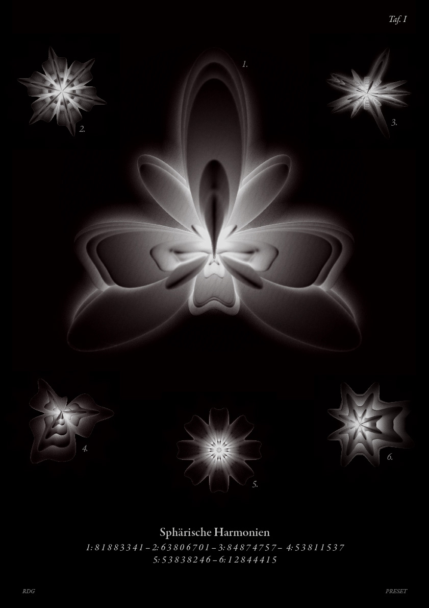
The following closed objects are commonly called spherical harmonics although they are only remotely related to the mathematical definition found in the solution to certain wave functions, most notable the eigenfunctions of angular momentum operators. The formula is quite simple, the form used here is based upon spherical (polar) coordinates (radius, theta, phi).
Where phi ranges from 0 to pi (lines of latitude), and theta ranges from 0 to 2 pi (lines of longitude), and r is the radius. The parameters m0, m1, m2, m3, m4, m5, m6, and m7 are all integers greater than or equal to 0.
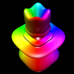 Implementation details The images here were created using OpenGL. While the parameters m0, m1, m2, m3, m4, m5, m6, m7 can range from 0 upwards, as the degree increases the objects become increasingly "pointed" and a large number of polygons are required to represent the surface faithfully. All the examples here have a maximum degree of 6. The maximum number of polygons used is 128 x 128 and most were only 64 x 64, that is, the theta and phi angles are split into 64 equal steps each. The C function that computes a point on the surface is
XYZ Eval(double theta,double phi, int *m)
{
   double r = 0;
   XYZ p;

   r += pow(sin(m[0]*phi),(double)m[1]);
   r += pow(cos(m[2]*phi),(double)m[3]);
   r += pow(sin(m[4]*theta),(double)m[5]);
   r += pow(cos(m[6]*theta),(double)m[7]);

   p.x = r * sin(phi) * cos(theta);
   p.y = r * cos(phi);
   p.z = r * sin(phi) * sin(theta);

   return(p);
}
The OpenGL snippet that creates the geometry is
   du = TWOPI / (double)resolution; /* Theta */
   dv = PI / (double)resolution;    /* Phi   */

   glBegin(GL_QUADS);
   for (i=0;i<resolution;i++) {
      u = i * du;
      for (j=0;j<resolution;j++) {
         v = j * dv;
         q[0] = Eval(u,v);
         n[0] = CalcNormal(q[0],
                           Eval(u+du/10,v),
                           Eval(u,v+dv/10));
         c[0] = GetColour(u,0.0,TWOPI,colourmap);
         glNormal3f(n[0].x,n[0].y,n[0].z);
         glColor3f(c[0].r,c[0].g,c[0].b);
         glVertex3f(q[0].x,q[0].y,q[0].z);

         q[1] = Eval(u+du,v);
         n[1] = CalcNormal(q[1],
                           Eval(u+du+du/10,v),
                           Eval(u+du,v+dv/10));
         c[1] = GetColour(u+du,0.0,TWOPI,colourmap);
         glNormal3f(n[1].x,n[1].y,n[1].z);
         glColor3f(c[1].r,c[1].g,c[1].b);
         glVertex3f(q[1].x,q[1].y,q[1].z);

         q[2] = Eval(u+du,v+dv);
         n[2] = CalcNormal(q[2],
                           Eval(u+du+du/10,v+dv),
                           Eval(u+du,v+dv+dv/10));
         c[2] = GetColour(u+du,0.0,TWOPI,colourmap);
         glNormal3f(n[2].x,n[2].y,n[2].z);
         glColor3f(c[2].r,c[2].g,c[2].b);
         glVertex3f(q[2].x,q[2].y,q[2].z);

         q[3] = Eval(u,v+dv);
         n[3] = CalcNormal(q[3],
                           Eval(u+du/10,v+dv),
                           Eval(u,v+dv+dv/10));
         c[3] = GetColour(u,0.0,TWOPI,colourmap);
         glNormal3f(n[3].x,n[3].y,n[3].z);
         glColor3f(c[3].r,c[3].g,c[3].b);
         glVertex3f(q[3].x,q[3].y,q[3].z);
      }
   }
   glEnd();
 Exercises for the reader
|