Spline Surface (in 3D)

Written by Paul Bourke
November 1996

Creating a spline surface involves taking the product of the same spline blending functions used for spline curves as follows

where the control points form a 2D array P_ij. Most of the properties of the spline curve also apply to spline surfaces. For example

The surface passes through the end (corner) points
The surface lies within the convex hull of the control points
The smoothness of the surface can be controlled and this can be done independently in both directions.
The resolution of the surface can be controlled and this can be different in each direction.

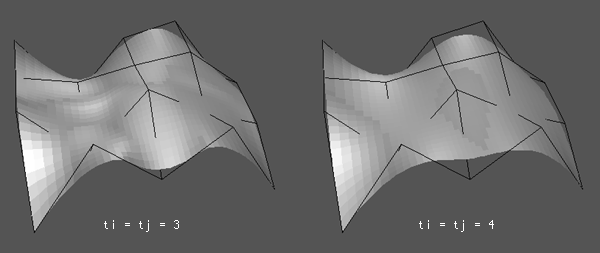
As an example the following show the surface given a 4x5 matrix of control points, degree 3 in both directions, the surface is sampled on a 30x40 grid.

Zero order continuity between spline surfaces is ensured if the control points along the joining edge are the same. First order continuity can be obtained by matching the control point slope across the boundary. This also applies to attempts to form a closed spline surface.

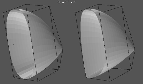
Forming a closed surface is easier if third order splines are being used because the surface is tangential to the end planes. In the following image the surface on the right starts and ends at the origin. The surface on the right has an extra control point so that the start and end planes have the same tangent.

C Source Example The following example show how to create a spline surface in the images above using GeomView.

/*
   Create an example of a spline surfaces
*/
#define NI 3
#define NJ 4
XYZ inp[NI+1][NJ+1];
#define TI 3
#define TJ 3
int knotsI[NI+TI+1];
int knotsJ[NJ+TJ+1];
#define RESOLUTIONI 30
#define RESOLUTIONJ 40
XYZ outp[RESOLUTIONI][RESOLUTIONJ];

int main(argc,argv)
int argc;
char **argv;
{
   int i,j,ki,kj;
   double intervalI,incrementI;
   double intervalJ,incrementJ;
   double bi,bj;

   /* Create a random surface */
   srandom(1111);
   for (i=0;i<=NI;i++) {
      for (j=0;j<=NJ;j++) {
         inp[i][j].x = i;
         inp[i][j].y = j;
         inp[i][j].z = (random() % 10000) / 5000.0 - 1;
      }
   }

   /* Step size along the curve */
   incrementI = (NI - TI + 2) / ((double)RESOLUTIONI - 1);
   incrementJ = (NJ - TJ + 2) / ((double)RESOLUTIONJ - 1);

   /* Calculate the knots */
   SplineKnots(knotsI,NI,TI);
   SplineKnots(knotsJ,NJ,TJ);

   intervalI = 0;
   for (i=0;i<RESOLUTIONI-1;i++) {
      intervalJ = 0;
      for (j=0;j<RESOLUTIONJ-1;j++) {
         outp[i][j].x = 0;
         outp[i][j].y = 0;
         outp[i][j].z = 0;
         for (ki=0;ki<=NI;ki++) {
            for (kj=0;kj<=NJ;kj++) {
               bi = SplineBlend(ki,TI,knotsI,intervalI);
               bj = SplineBlend(kj,TJ,knotsJ,intervalJ);
               outp[i][j].x += (inp[ki][kj].x * bi * bj);
               outp[i][j].y += (inp[ki][kj].y * bi * bj);
               outp[i][j].z += (inp[ki][kj].z * bi * bj);
            }
         }
         intervalJ += incrementJ;
      }
      intervalI += incrementI;
   }
   intervalI = 0;
   for (i=0;i<RESOLUTIONI-1;i++) {
      outp[i][RESOLUTIONJ-1].x = 0;
      outp[i][RESOLUTIONJ-1].y = 0;
      outp[i][RESOLUTIONJ-1].z = 0;
      for (ki=0;ki<=NI;ki++) {
          bi = SplineBlend(ki,TI,knotsI,intervalI);
          outp[i][RESOLUTIONJ-1].x += (inp[ki][NJ].x * bi);
          outp[i][RESOLUTIONJ-1].y += (inp[ki][NJ].y * bi);
          outp[i][RESOLUTIONJ-1].z += (inp[ki][NJ].z * bi);
      }
      intervalI += incrementI;
   }
   outp[i][RESOLUTIONJ-1] = inp[NI][NJ];
   intervalJ = 0;
   for (j=0;j<RESOLUTIONJ-1;j++) {
      outp[RESOLUTIONI-1][j].x = 0;
      outp[RESOLUTIONI-1][j].y = 0;
      outp[RESOLUTIONI-1][j].z = 0;
      for (kj=0;kj<=NJ;kj++) {
          bj = SplineBlend(kj,TJ,knotsJ,intervalJ);
          outp[RESOLUTIONI-1][j].x += (inp[NI][kj].x * bj);
          outp[RESOLUTIONI-1][j].y += (inp[NI][kj].y * bj);
          outp[RESOLUTIONI-1][j].z += (inp[NI][kj].z * bj);
      }
      intervalJ += incrementJ;
   }
   outp[RESOLUTIONI-1][j] = inp[NI][NJ];

   printf("LIST\n");

   /* Display the surface, in this case in OOGL format for GeomView */
   printf("{ = CQUAD\n");
   for (i=0;i<RESOLUTIONI-1;i++) {
      for (j=0;j<RESOLUTIONJ-1;j++) {
        printf("%g %g %g 1 1 1 1\n",
            outp[i][j].x,    outp[i][j].y,    outp[i][j].z);
        printf("%g %g %g 1 1 1 1\n",
            outp[i][j+1].x,  outp[i][j+1].y,  outp[i][j+1].z);
        printf("%g %g %g 1 1 1 1\n",
            outp[i+1][j+1].x,outp[i+1][j+1].y,outp[i+1][j+1].z);
        printf("%g %g %g 1 1 1 1\n",
            outp[i+1][j].x,  outp[i+1][j].y,  outp[i+1][j].z);
      }
   }
   printf("}\n");

   /* Control point polygon */
   for (i=0;i<NI;i++) {
      for (j=0;j<NJ;j++) {
         printf("{ = SKEL 4 1  \n");
         printf("%g %g %g \n",inp[i][j].x,inp[i][j].y,inp[i][j].z);
         printf("%g %g %g \n",inp[i][j+1].x,inp[i][j+1].y,inp[i][j+1].z);
         printf("%g %g %g \n",inp[i+1][j+1].x,inp[i+1][j+1].y,inp[i+1][j+1].z);
         printf("%g %g %g \n",inp[i+1][j].x,inp[i+1][j].y,inp[i+1][j].z);
         printf("5 0 1 2 3 0\n");
         printf("}\n");
      }
   }
}

Spline curves (in 3D)

Written by Paul Bourke
November 1996

Spline curves originate from flexible strips used to create smooth curves in traditional drafting applications. Much like Bezier curves they are formed mathematically from piecewise approximations of cubic polynomial functions with zero, first and second order continuity.

B-Splines are one type of spline that are perhaps the most popular in computer graphics applications, they are defined as follows:
If we have N+1 control points P_k we can derive a continuous function P(v) as

where N(v) are called blending functions, u_k are known as break points, where they occur on the curve are known as knots. There are a number of possible options for the knot positions, for example a uniform spacing where u_k = k. More commonly the following function is chosen

The blending functions are defined as

Such curves have many advantages

Changes to a control point only affects the curve in that locality

Any number of points can be added without increasing the degree of the polynomial.

As with Bezier curves adding multiple points at or near a single position draws the curve towards that position.

Closed curves can be created by making the first and last points the same, although continuity will not be maintained automatically.

B-Splines lie in the convex hull of the control points.

There is another curve in the family called Beta-Splines which have additional parameters beta1 and beta2 which adjust the shape relative to the convex hull. B-Splines are subsets of Beta-Splines.

The following example (created with the source below) shows the spline through 4 control points, with degree t = 2, 3, and 4. t = 2 is just linear interpolation, as the degree increases the smoother the curve becomes.

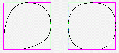
The pink line shows the polygon formed by the control points, the white line is the spline curve. Note that the curve lies within the convex hull of the points. Note also that the tangent of the curve at the endpoints is the same as the slope of the line between the first two or last two control points. This makes for convenient matching of the curve between sections. For example in the following the spline on the left has control points starting and ending at the origin. The curve on the right has control points on the same square but the start and end control point is along the bottom edge and the slope of the first two and last two control points is the same.

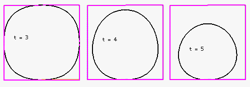
Unfortunately the curve always passes through the first and last point. The following has the same control points as for the curve on the right above but for increasing values of the degree, t.

Splines of degree 3 are by far the most commonly used in practice. Except for the first edge and last edge of the control point polygon these splines touch the midpoint of each other edge. If the control point polygon is concave the spline passes through the midpoint, if the polygon is concave the spline is tangential at the edge midpoint.

C Source Code

In what follows it will assumed there are n + 1 control points, P_k where k ranges from 0 to n. The parameter t determines the order of the polynomials used for the blending function, typically 3 or 4.
The routines presented here are for 3 dimensions but can be readily extended into higher dimensions.

Following are three functions which implement spline curves, at the end there is a small demonstration program which calls these routines to create the image shown earlier.

/*
   This returns the point "output" on the spline curve.
   The parameter "v" indicates the position, it ranges from 0 to n-t+2
   
*/
void SplinePoint(int *u,int n,int t,double v,XYZ *control,XYZ *output)
{
   int k;
   double b;

   output->x = 0;
   output->y = 0;
   output->z = 0;

   for (k=0;k<=n;k++) {
      b = SplineBlend(k,t,u,v);
      output->x += control[k].x * b;
      output->y += control[k].y * b;
      output->z += control[k].z * b;
   }
}

/*
   Calculate the blending value, this is done recursively.
   
   If the numerator and denominator are 0 the expression is 0.
   If the deonimator is 0 the expression is 0
*/
double SplineBlend(int k,int t,int *u,double v)
{
   double value;

   if (t == 1) {
      if ((u[k] <= v) && (v < u[k+1]))
         value = 1;
      else
         value = 0;
   } else {
      if ((u[k+t-1] == u[k]) && (u[k+t] == u[k+1]))
         value = 0;
      else if (u[k+t-1] == u[k]) 
         value = (u[k+t] - v) / (u[k+t] - u[k+1]) * SplineBlend(k+1,t-1,u,v);
      else if (u[k+t] == u[k+1])
         value = (v - u[k]) / (u[k+t-1] - u[k]) * SplineBlend(k,t-1,u,v);
     else
         value = (v - u[k]) / (u[k+t-1] - u[k]) * SplineBlend(k,t-1,u,v) + 
                 (u[k+t] - v) / (u[k+t] - u[k+1]) * SplineBlend(k+1,t-1,u,v);
   }
   return(value);
}

/*
   The positions of the subintervals of v and breakpoints, the position
   on the curve are called knots. Breakpoints can be uniformly defined
   by setting u[j] = j, a more useful series of breakpoints are defined
   by the function below. This set of breakpoints localises changes to
   the vicinity of the control point being modified.
*/
void SplineKnots(int *u,int n,int t)
{
   int j;

   for (j=0;j<=n+t;j++) {
      if (j < t)
         u[j] = 0;
      else if (j <= n)
         u[j] = j - t + 1;
      else if (j > n)
         u[j] = n - t + 2;	
   }
}

/*-------------------------------------------------------------------------
   Create all the points along a spline curve
   Control points "inp", "n" of them.
   Knots "knots", degree "t".
   Ouput curve "outp", "res" of them.
*/
void SplineCurve(XYZ *inp,int n,int *knots,int t,XYZ *outp,int res)
{
   int i;
   double interval,increment;

   interval = 0;
   increment = (n - t + 2) / (double)(res - 1);
   for (i=0;i<res-1;i++) {
      SplinePoint(knots,n,t,interval,inp,&(outp[i]));
      interval += increment;
   }
   outp[res-1] = inp[n];
}

/*
   Example of how to call the spline functions
	Basically one needs to create the control points, then compute
   the knot positions, then calculate points along the curve.
*/
#define N 3
XYZ inp[N+1] = {0.0,0.0,0.0,   1.0,0.0,3.0,   2.0,0.0,1.0,   4.0,0.0,4.0};
#define T 3
int knots[N+T+1];
#define RESOLUTION 200
XYZ outp[RESOLUTION];

int main(int argc,char **argv)
{
   int i;

   SplineKnots(knots,N,T);
   SplineCurve(inp,N,knots,T,outp,RESOLUTION);

   /* Display the curve, in this case in OOGL format for GeomView */
   printf("LIST\n");
   printf("{ = SKEL\n");
   printf("%d %d\n",RESOLUTION,RESOLUTION-1);
   for (i=0;i<RESOLUTION;i++)
      printf("%g %g %g\n",outp[i].x,outp[i].y,outp[i].z);
   for (i=0;i<RESOLUTION-1;i++)
      printf("2 %d %d 1 1 1 1\n",i,i+1);
   printf("}\n");

   /* The axes */
   printf("{ = SKEL 3 2  0 0 4  0 0 0  4 0 0  2 0 1 0 0 1 1 2 1 2 0 0 1 1 }\n");

   /* Control point polygon */
   printf("{ = SKEL\n");
   printf("%d %d\n",N+1,N);
   for (i=0;i<=N;i++)
      printf("%g %g %g\n",inp[i].x,inp[i].y,inp[i].z);
   for(i=0;i<N;i++)
      printf("2 %d %d 0 1 0 1\n",i,i+1);
   printf("}\n");

}

References

Chankin, G. An algorithm for high speed curve generation. Computer Graphics and Image Processing, 3 (1974), 346-349

Riesenfeld, R. On Chaikin's algorithm. IEEE Computer Graphics and Applications, 4, 3 (1975) 304-310