Fisheye lens correctionWritten by Paul BourkeOriginal November 2016, data being updated regularly
See also: fisheyerectify.pdf (March 2018)
The source code implementing the projections below is only available on request for a small fee. It includes a demo application and an invitation to convert an image of your choice to verify the code does what you seek. For more information please contact the author.
A normal lens has pincushion or barrel distortion which can be corrected for to give a perfect perspective projection, a pin-hole camera. This is called "rectification" and is often applied before any warp/stitch/blending is applied, for example, in panoramic photography. In the same way there is a perfect circular fisheye projection, that is, one in which the distance r from the center of the fisheye circle is linearly proportional to the latitude of the corresponding 3D vector. In the following, along any radial line on the fisheye (left), two points separated by the same pixel distance, correspond to the same angular distance (right). 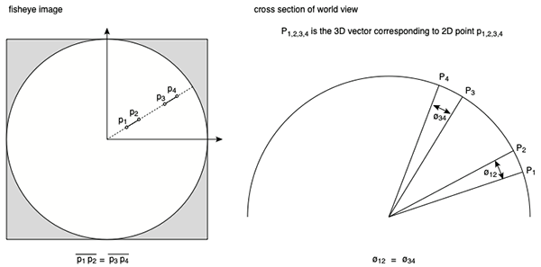
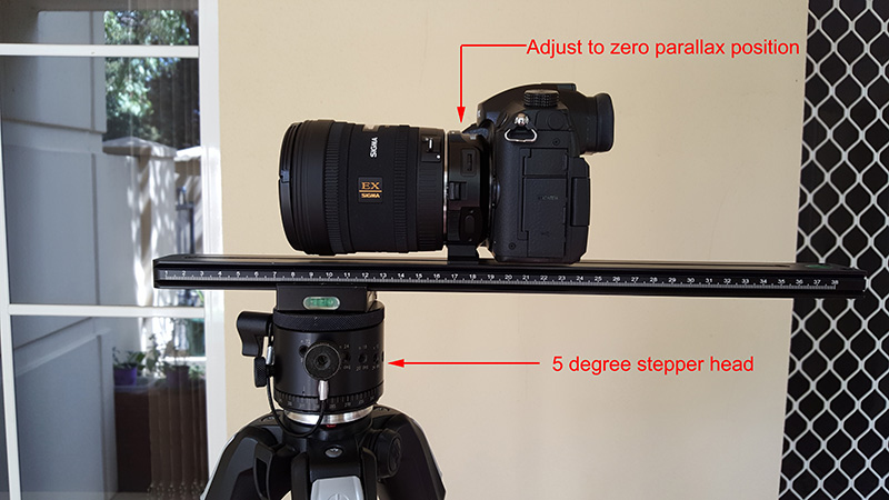
Such a fisheye lens is often referred to as a "tru-theta" lens and while such lenses can and have been manufactured, in real life and for lower cost lenses the relationship is non-linear. The non-linearity normally occurs towards the periphery of the fisheye and results in a compression effect. In many cases the lens manufacturer can supply data for the curve relating "r", the distance on the sensor or fisheye circular image, to latitude (often called "field angle") of the 3D vector corresponding to that radius. In some cases for high grade lenses the manufacturer will supply curves for the particular lens in question, an acknowledgement that lenses can vary typically by 5% in the manufacturing process. In the situation where no such data is available one needs to construct a rig that will allow the angles to be measured. The approach to correcting for the non-linear relationship is to fit a suitable polynomial to the data points relating "r" to latitude. A general function for the latitude φ might be
Since the fisheye is assumed to be radially symmetric and r=0 is the center of the fisheye corresponding to a latitude of 0, a0 is zero. In practice the highest order polynomial needed for the fitting is usually n=3, in some extreme examples a 4th order (n=4) is required. So the polynomial for a least squares fit is
The case where the fisheye already has a linear relationship would be a1 = φmax / rmax, a2 = 0, a3 = 0, and a4 = 0. Where φmax is the half the circular fisheye angle and rmax the radius on the image or sensor corresponding to φmax. Noting that the r is often normalised to 1, in which case rmax = 1. In order to correct a source image, the software actually performs the mapping in the reverse direction. That is, one considers each position on the destination image and derives the matching position and therefore best RGB value in the source image. As such what one actually needs to compute is the radius as a function of field angle, the inverse function of the equations presented earlier, in other words:
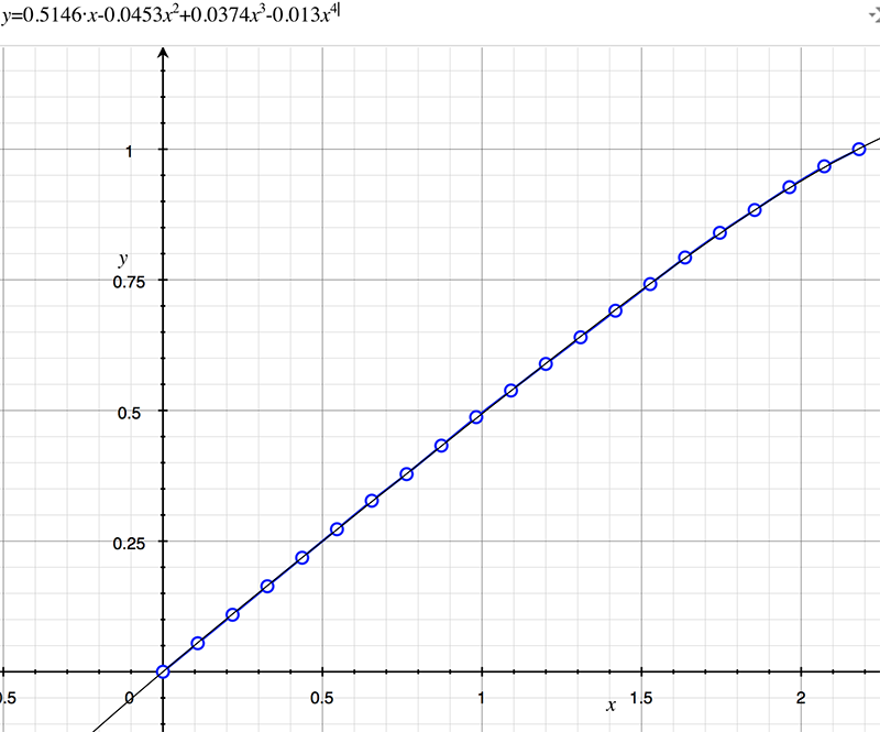
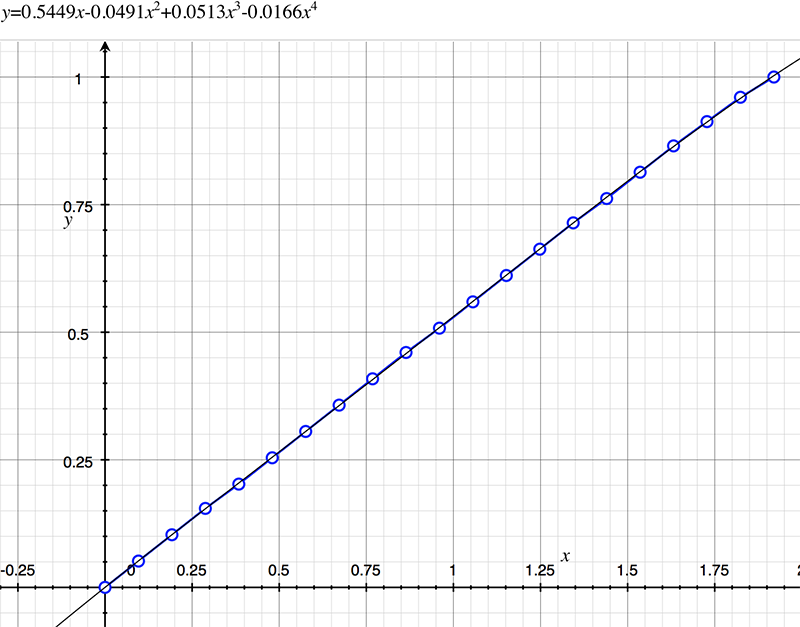
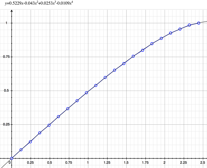
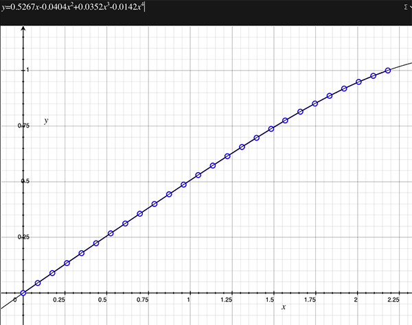
As an example, the following data relating field angle to distance on the sensor is illustrated below for a 190 degree fisheye The samples are in blue and the fitted curve is shown in grey, The red line shows the relationship for a perfectly linear fisheye, this is also the relationship after the correction is performed. The horizontal axis is the field of view (field angle) in radians and the vertical axis is normalised fisheye image coordinates, that is, the radius is unity for the field of view at the fisheye circle. 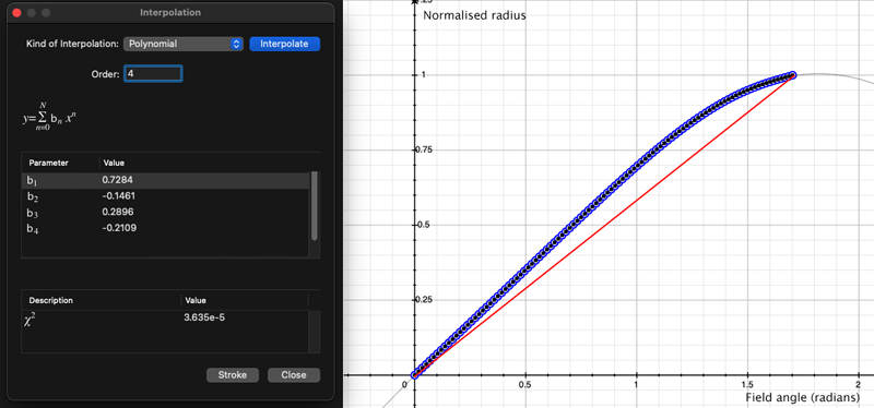
Usage
The usage string for the command line application is shown below. The main option is -p where the fitted parameters are provided. The center of the fisheys circle (-c) and the radius (-r) mean that images directly off the camera sensor can be transformed without first cropping it square. Rotations can be performed about any axis and in any order. The coordinate system is right handed, y is forward along the optical axis of the fisheye (rotation in y is a roll), z is upwards (rotation about z is a pan), and the x axis is to the right (rotation about x is a tilt). Usage: fishcorrect [options] imagefile Options -w n sets the output fisheye width, default: same as source fisheye -a n sets antialiasing level, default: 2 -s n source fisheye field of view (degrees), default: 180 -t n output fisheye field of view (degrees), default: same as source -c x y source fisheye center, default: center of image -r n source fisheye radius, default: half the fisheye image width -x n tilt angle (degrees), default: 0 -y n roll angle (degrees), default: 0 -z n pan angle (degrees), default: 0 -ox n fisheye offset amount in x axis, default: 0 -oy n fisheye offset amount in y axis, default: 0 -oz n fisheye offset amount in z axis, default: 0 -p n n n n fourth order correction terms, default: no correction -o s output filename, default: derived from input file -d debug mode
Updates
It should be noted that the utility described here transforms a fisheye into a linear fisheye. More often than not one is converting the fisheye into some other mapping, perhaps an equirectangular (fish2sphere) or extracting a perspective projection (fish2persp). In these cases the non-linearity of the fisheye should be incorporated directly into the equations for those mappings, rather than being performed as a separate image transformation process.. Example
The following image is captured with a 210 degree fisheye which has quite significant compression towards the rim. 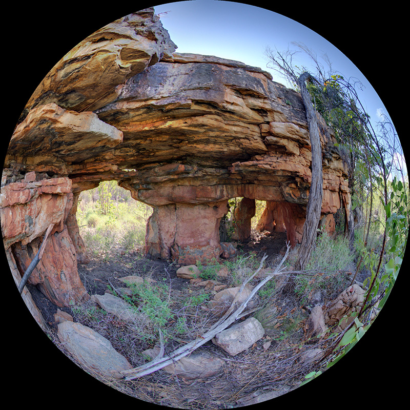
The following is the undistorted version, that is, radius on the fisheye images is now proportional to latitude. 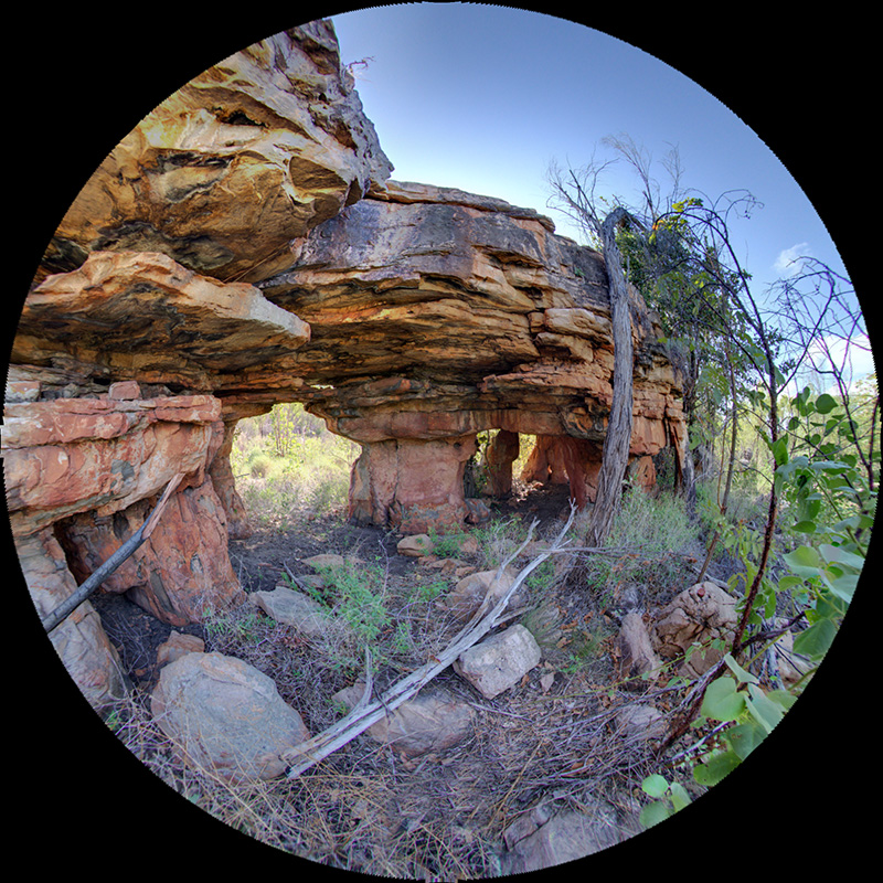
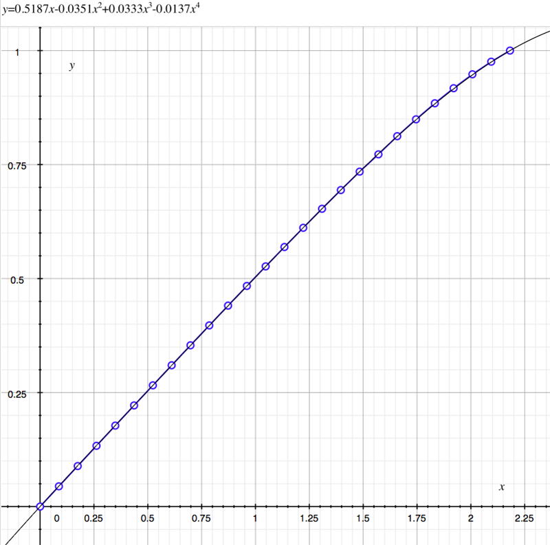
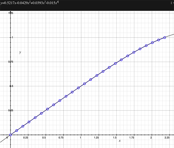
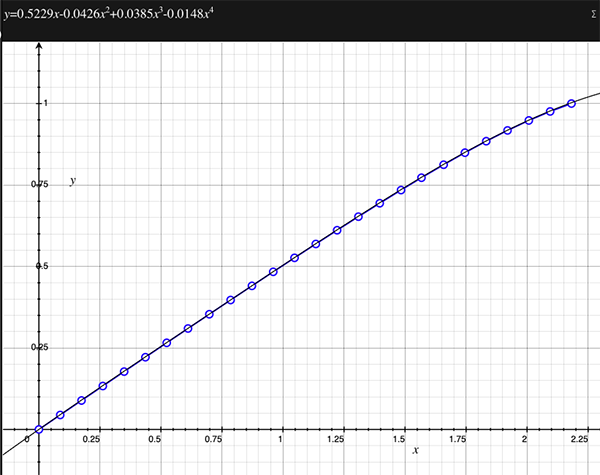
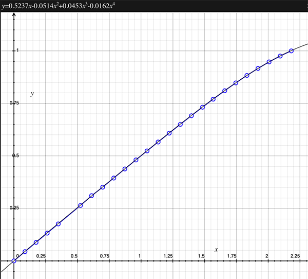
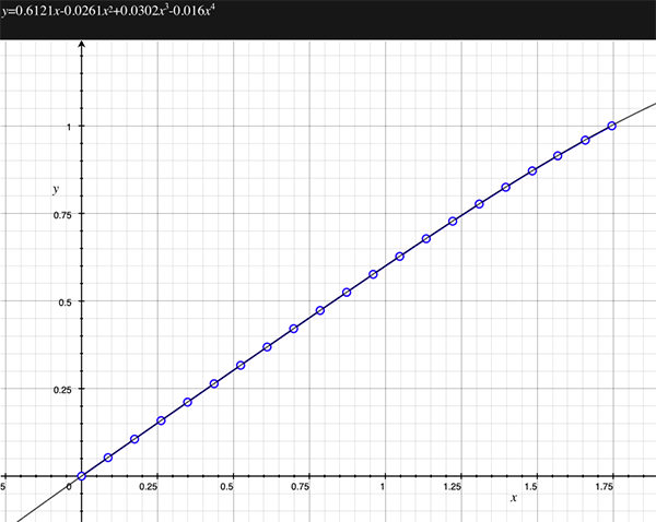
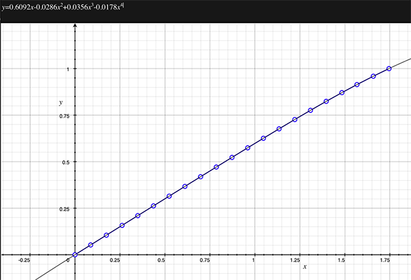
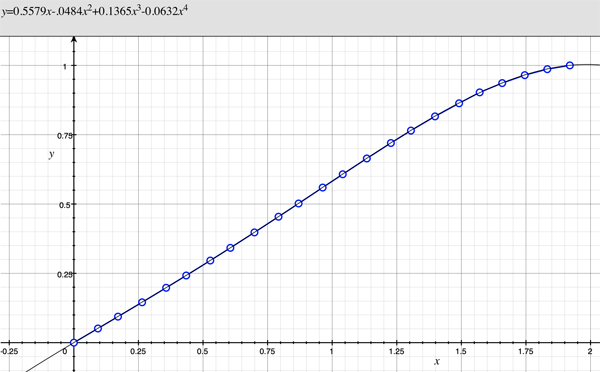
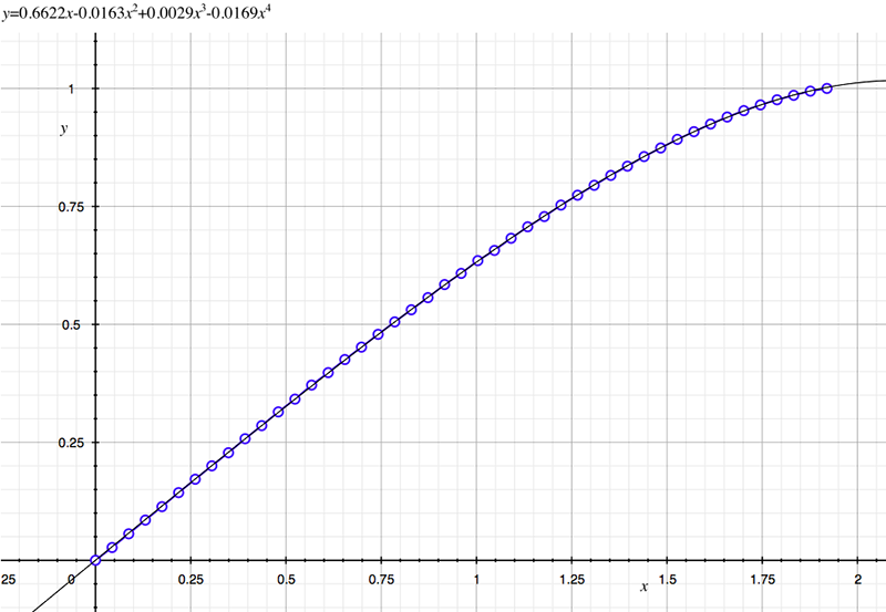
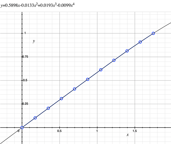
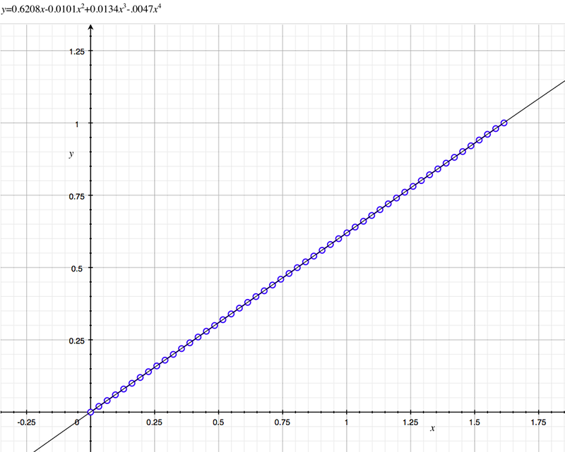
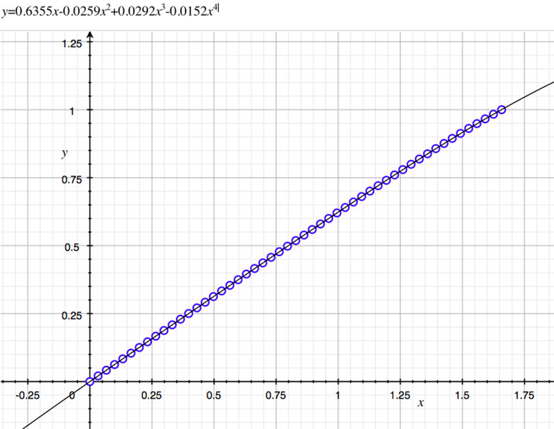
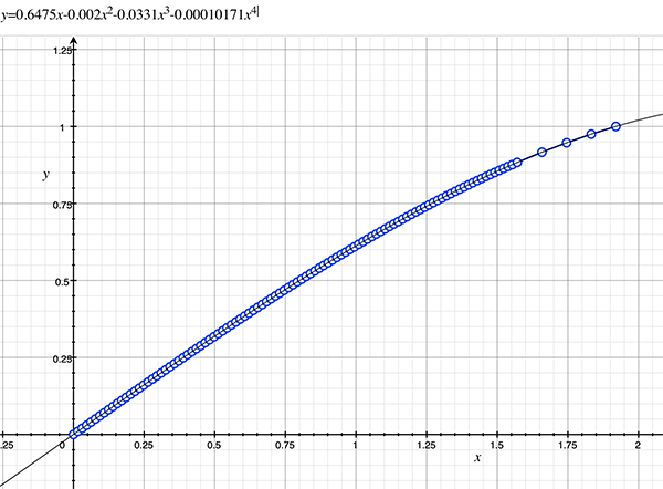
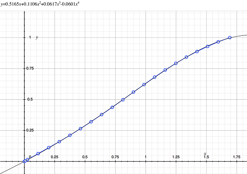
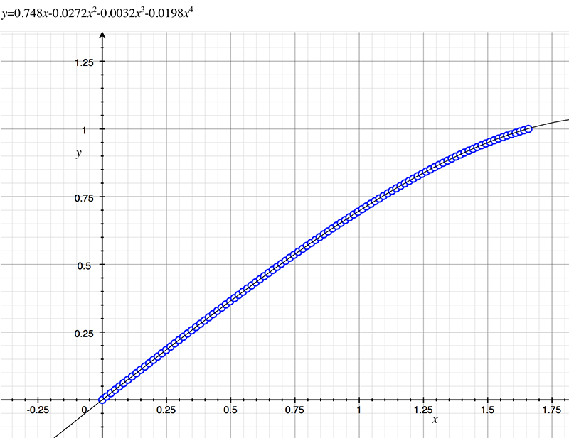
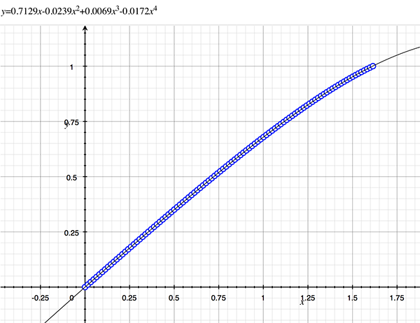
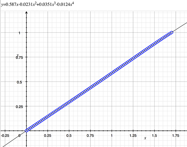
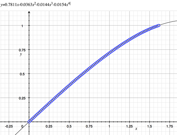
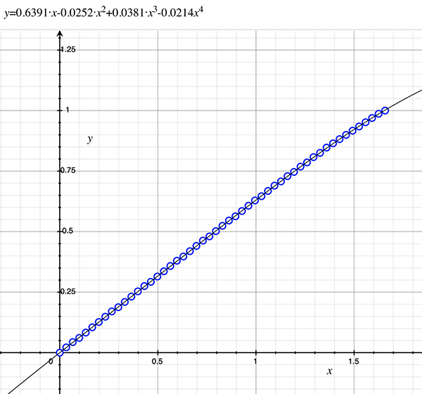
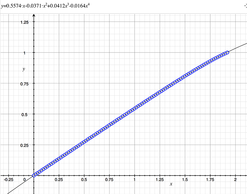
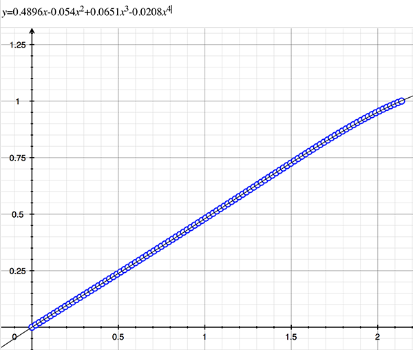
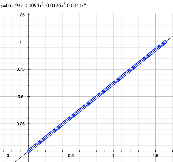
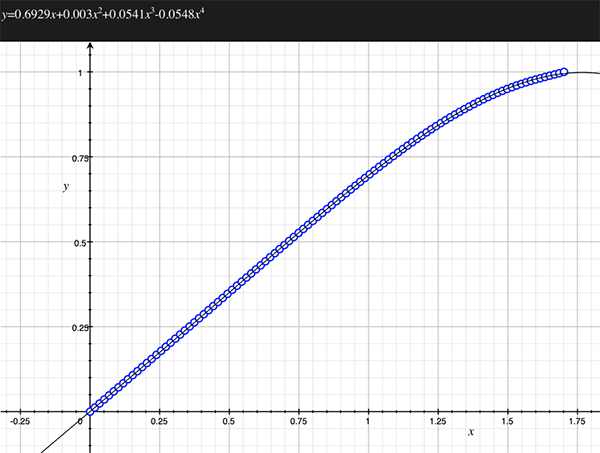
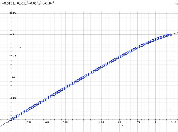
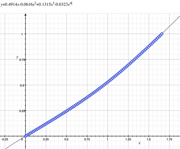
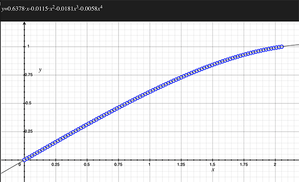
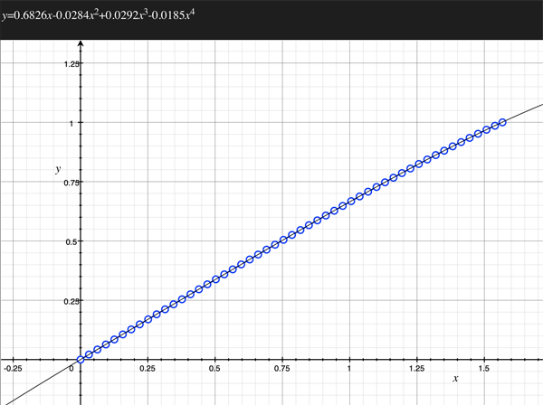
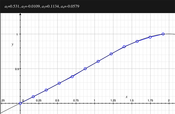
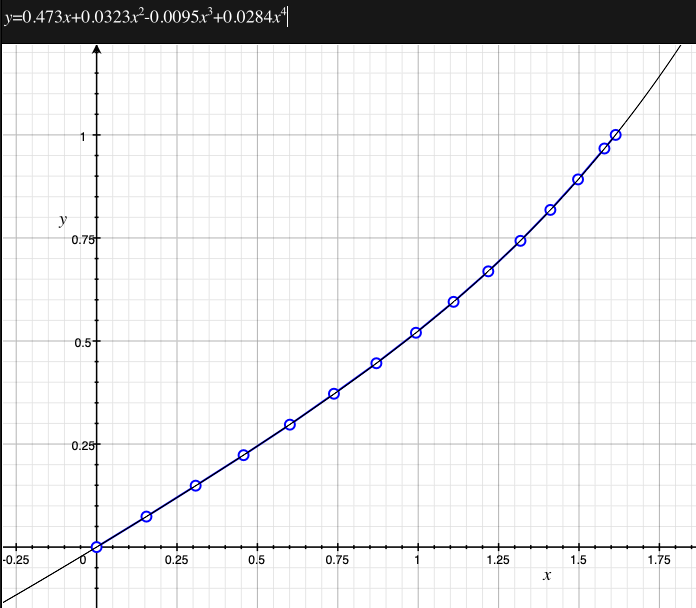
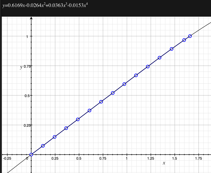
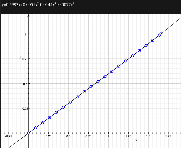
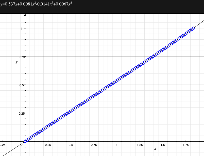
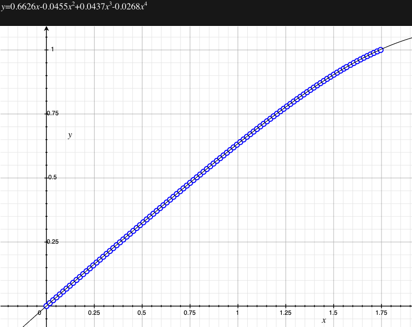
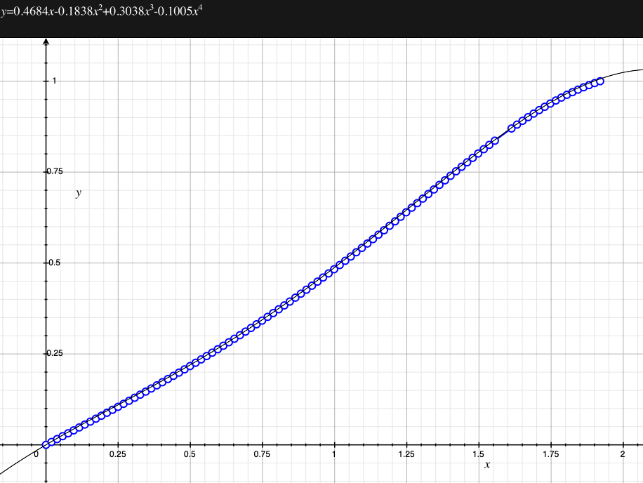
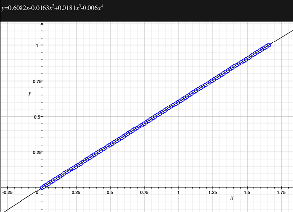
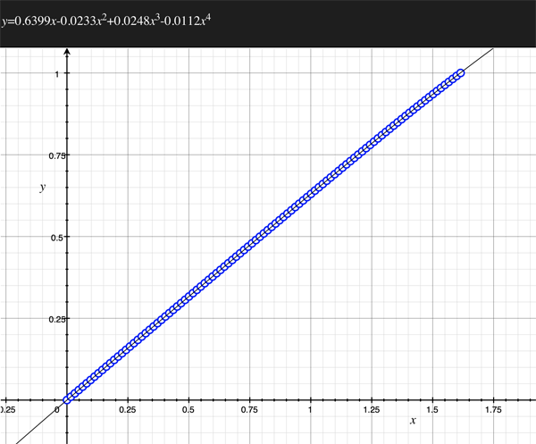
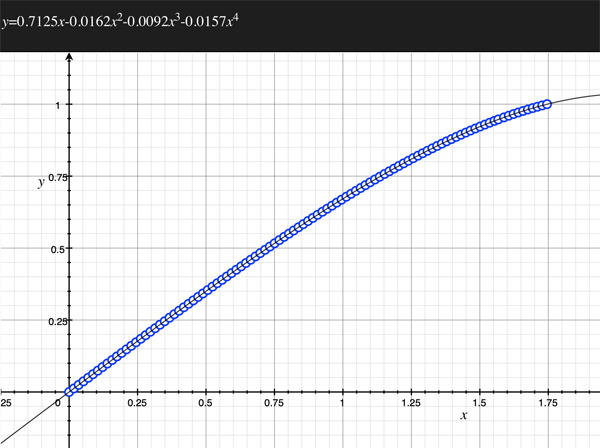
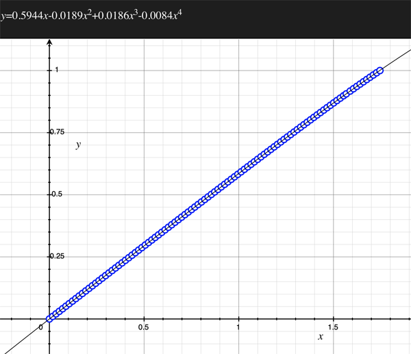
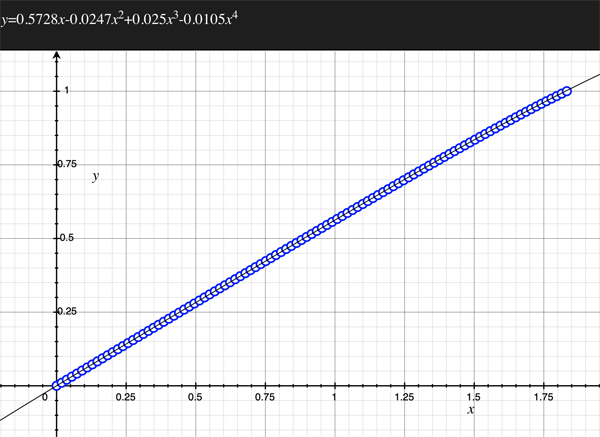
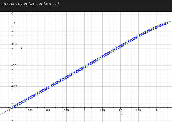
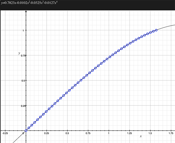
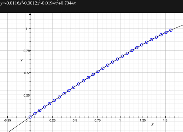
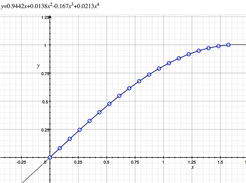
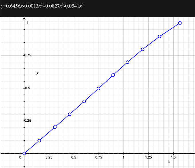
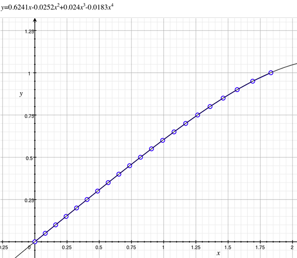
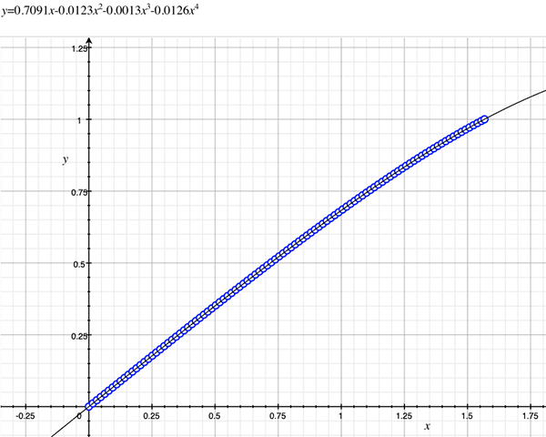
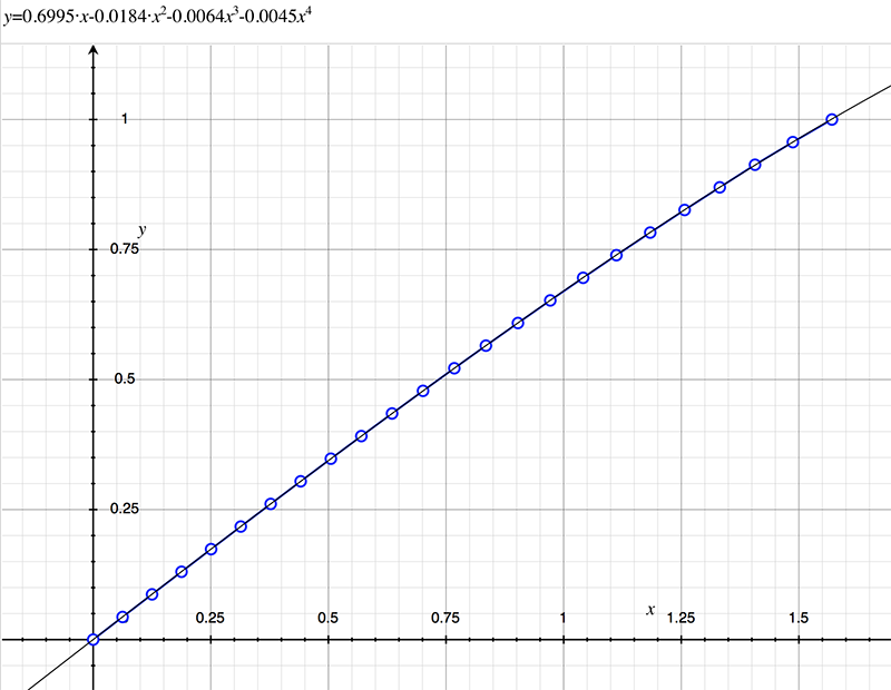
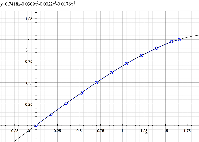
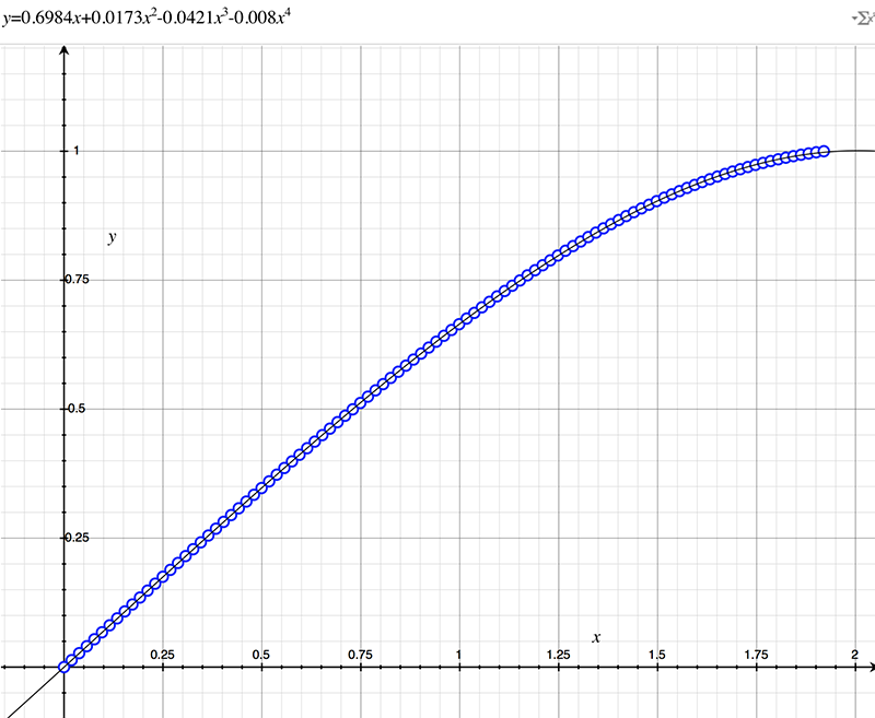
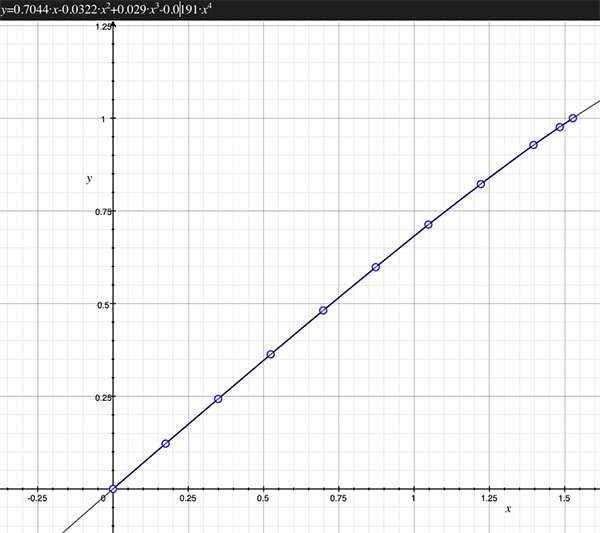
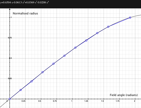
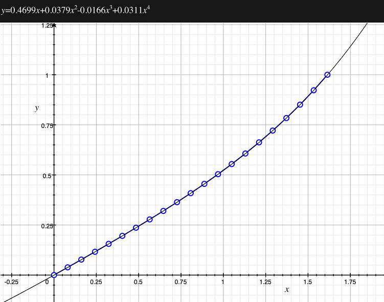
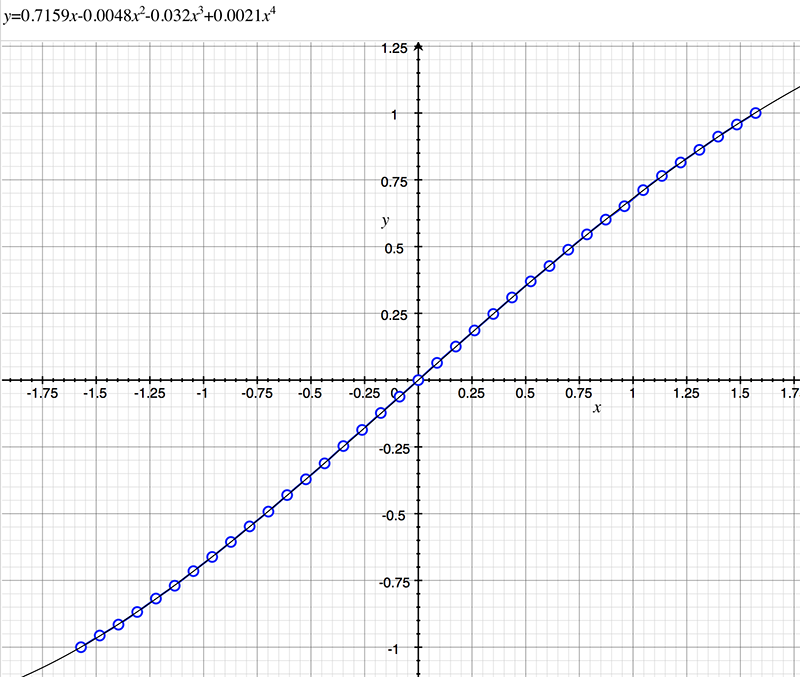
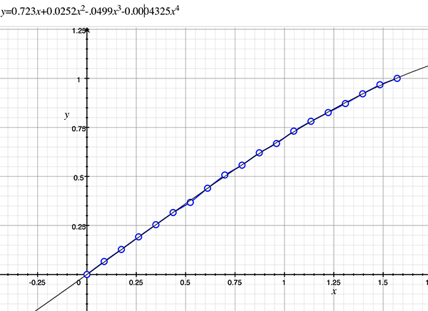
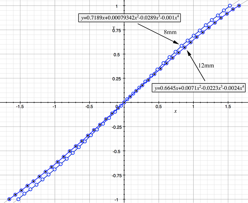
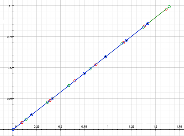
In the remainder of this document the curves and polynomial correction values for various fisheye lenses are presented. These are collected by the author as lenses and/or data are made available. The functions are all 4th order. Graphs are radians horizontally, and normalised radius of the position on the fisheye image (sensor) vertically. Entaniya
iZugar
Meike
Sunex
Aico
Evetar
Arducam
Computar
Commonlands
Xiamen Alaud Optical
Others
|
