Gauss Map tetrahedron 3D IFSAlternative title: Rendering IFS (Iterated Function System) in a volume rendererWritten by Paul BourkeSubmitted by Roger Bagula May 2014 See also: Visualising volumetric fractals
An Iterated Function System (IFS) is a series where the next point in the series is a function of the last point. where
In two dimensions the points are represented visually by pixels on the image plane, a very well known example is the IFS fern. Colour can be added in a number of ways. One is to treat the discrete image plane as a histogram and points falling within the bounds of a pixel are accumulated, the resulting height field can be colour coded. An example of this can be seen in the IFS popcorn fractal. Many IFS are made up from a number of functions one of which is chosen at random to determine the next point in the series. These functions may be selected each with a different probability. The IFS dragon is an example where there are two equations for determining the next point in the series and they are chosen with probability 0.8 and 0.2. In 3 dimensions the point nature of IFS makes direct graphical representations more difficult. In short, a few million points drawn as little dots or spheres is generally an unattractive and uninformative image. An example of a million points as small spheres for the IFS demonstrated here is shown below. 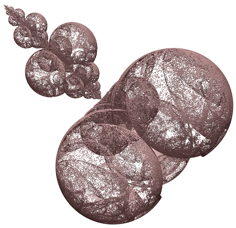
The approach used here is to map the IFS points into a discrete regular volume and use a volume renderer, in this case Drishti, to visualise the IFS attractor. In essence leveraging the rich history and software for volume visualisation. The particular IFS used to illustrate this approach is defined by the following 5 equations, on each iteration one function is chosen at random with equal probability. The resulting "surface" is the attractor of the system. pn+1 = ( 2 pn.x / (1 + pn2.x + pn2.y), 2 pn.y / (1 + pn2.x + pn2.y), (1 - pn2.x - pn2.y) / (1 + pn2.x + pn2.y) ) + (-1,-1,0)pn+1 = ( (1 - pn2.z - pn2.y) / (1 + pn2.z + pn2.y), 2 pn.y / (1 + pn2.z + pn2.y), 2 pn.z / (1 + pn2.z + pn2.y) ) + (0,-1,-1) pn+1 = ( 2 pn.x / (1 + pn2.z + pn2.x), (1 - pn2.z - pn2.x / (1 + pn2.z + pn2.x), 2 pn.z / (1 + pn2.z + pn2.x) ) + (-1,0,-1) pn+1 = pn / 2 pn+1 = pn / 2 + (1,1,1)
The rendering below is 500 million points sampled into a 5123 volume. The points falling within a voxel are accumulated and the volume visualisation can shade the more frequently traversed points on the attractor. The discrete voxel nature of the rendering is clear, while this can be reduced by increasing the volume resolution the gains are modest when compared to the effect on data size and interactivity. In particular, to just double the resolution incurs a 8 fold penalty. 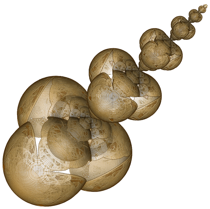
One way to smooth the edges of the attractor boundary is to add points to the volume with a point spread function, that is, when a point is added it also makes a contribution not only to the voxel containing the point but also to the neighbouring voxels. The addition to the surrounding voxels is some monotonically decreasing function of radius. The following is an example where the radial weighting is 1 / (1 + di2 + dj2 + dk2) where (di,dj,dk) is the voxel distance from the (i,j,k) voxel containing the point being added. The range of (di,dj,dk) in this case is -2 <= (di,dj,dk) <= 2. Note this is different to just smoothing the attractor voxels as a post production process. 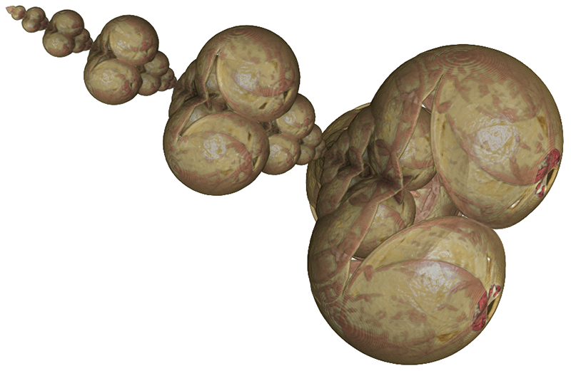
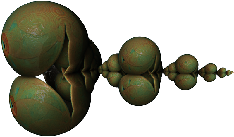
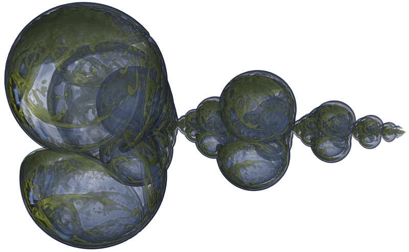
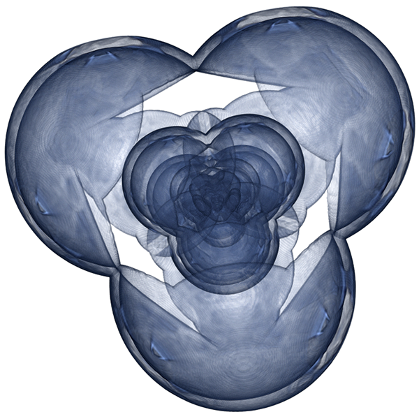
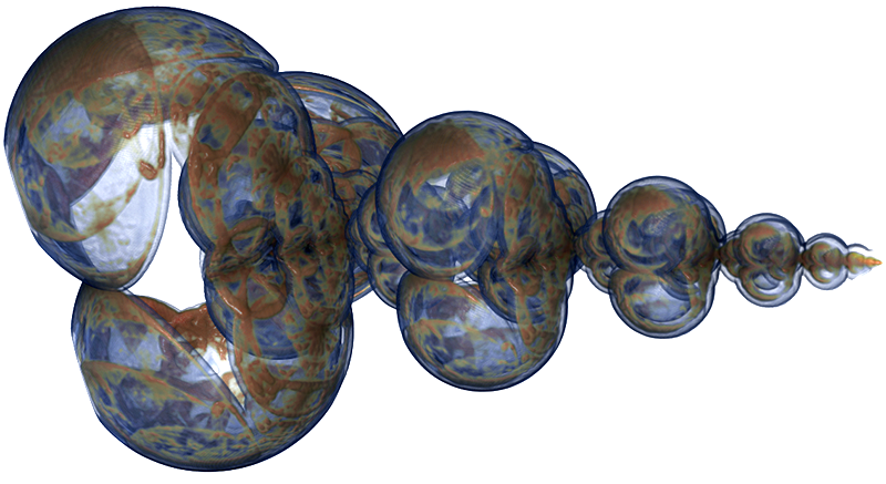
Other renderings follow from different sides and applying different transfer functions. 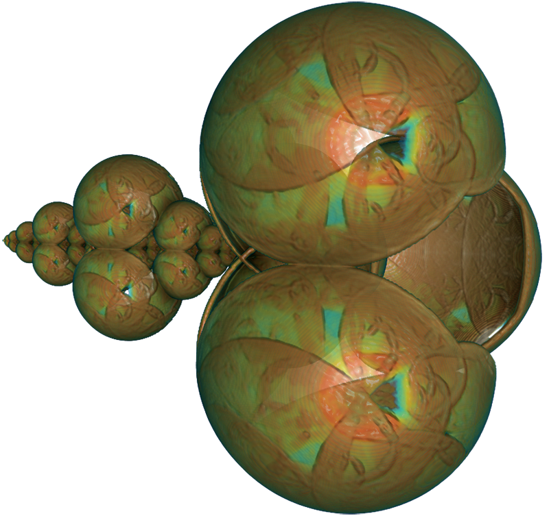
|