CONREC
A Contouring Subroutine
Written by Paul Bourke
July 1987
Source code

The famous BYTE magazine,
in which the algorithm appeared.
At least the algorithm survived.
Introduction
This article introduces a straightforward method of contouring some surface
represented as a regular triangular mesh.
Contouring aids in visualizing three dimensional surfaces on a two dimensional
medium (on paper or in this case a computer graphics screen). Two most common
applications are displaying topological features of an area on a map or the air
pressure on a weather map. In all cases some parameter is plotted as a function
of two variables, the longitude and latitude or x and y axis. One problem with
computer contouring is the process is usually CPU intensive and the algorithms
often use advanced mathematical techniques making them susceptible to error.
CONREC
To do contouring in software you need to describe the data surface and the
contour levels you want to have drawn. The software given this information must
call the algorithm that calculates the line segments that make up a contour
curve and then plot these line segments on whatever graphics device is
available.
CONREC satisfies the above description, it is relatively simple to implement,
very reliable, and does not require sophisticated programming techniques or a
high level of mathematics to understand how it works.
The input parameters to the CONREC subroutine are as follows :
The number of horizontal and vertical data points designated iub and jub.
The number of contouring levels, nc.
A one dimensional array z(0:nc-1) that saves as a list of the contour levels
in increasing order. (The order of course can be relaxed if the program will
sort the levels)
A two dimensional array d(0:iub,0:jub) that contains the description of the
data array to be contoured. Each element of the array is a sample of the
surface being studied at a point (x,y)
Two, one dimensional arrays x(0:iub) and y(0:jub) which contain the
horizontal and vertical coordinates of each sample point. This allows for a
rectangular grid of samples.
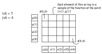
Figure 1
Illustrates some of the above input parameters.
The contouring subroutine CONREC does not assume anything about the device that
will be used to plot the contours. It instead expects a user written subroutine
called VECOUT. CONREC calls VECOUT with the horizontal and vertical coordinates
of the start and end coordinates of a line segment along with the contour level
for that line segment. In the simplest case this is very similar the the usual
LINE (x1,y1)-(x2,y2) command in BASIC. See the source code listing below.
Algorithm
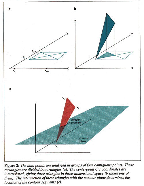
As already mentioned the samples of the three dimensional surface are stored in
a two dimensional real array. This rectangular grid is considered four points
at a time, namely the rectangle d(i,j), d(i+1,j), d(i,j+1), and d(i+1,j+1). The
centre of each rectangle is assigned a value corresponding to the average
values of each of the four vertices. Each rectangle is in turn divided into
four triangular regions by cutting along the diagonals. Each of these
triangular planes may be bisected by horizontal contour plane. The intersection
of these two planes is a straight line segment, part of the the contour curve
at that contour height.
Depending on the value of a contour level with respect to the height at the
vertices of a triangle, certain types of contour lines are drawn. The 10
possible cases which may occur are summarised below
a) All the vertices lie below the contour level.
b) Two vertices lie below and one on the contour level.
c) Two vertices lie below and one above the contour level.
d) One vertex lies below and two on the contour level.
e) One vertex lies below, one on and one above the contour level.
f) One vertex lies below and two above the contour level.
g) Three vertices lie on the contour level.
h) Two vertices lie on and one above the contour level.
i) One vertex lies on and two above the contour level.
j) All the vertices lie above the contour level.
In cases a, b, i and j the two planes do not intersect, ie: no line need be
drawn. For cases d and h the two planes intersect along an edge of the triangle
and therefore line is drawn between the two vertices that lie on the contour
level. Case e requires that a line be drawn from the vertex on the contour
level to a point on the opposite edge. This point is determined by the
intersection of the contour level with the straight line between the other two
vertices. Cases c and f are the most common situations where the line is drawn
from one edge to another edge of the triangle. The last possibility or case g
above has no really satisfactory solution and fortunately will occur rarely
with real arithmetic.
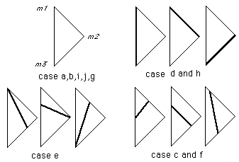
Figure 2
Example
As a simple example consider one triangle with vertices labelled m1,m2 and m3
with heights 0, 2 and 3 respectively
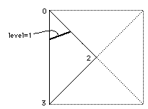
Figure 3 Summary of the possible line orientations.
To calculate where a contour line at a height of 1 should be drawn, it can be
seen that this is case f described earlier. Level 1 intersects line segment
m1-m2 half the way along and it intersects line segment m1-m3 one third of the
way along. A line segment is drawn between these two points. Each rectangular
mesh cell is treated this way.
Subroutine
In summary, CONREC takes each rectangle of adjacent data points and splits it
into 4 triangles after choosing the height at the centre of the rectangle. For
each of the triangles the line segment resulting from the intersection with
each contour plane. A routine is then called with the starting and stopping
coordinates of the line segment.
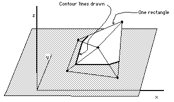
Figure 4
An attempt is made at optimization by checking first to
see if there are any contour levels within the present rectangle and second
that there are some contour levels within the present triangle. The indices i
and j are used to step through each rectangle in turn, k refers to each contour
level and m to the four triangles in each rectangle.
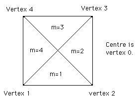
Figure 5
Some of the notation used for identifying the rectangles and
triangles in the subroutine.
Note that for large arrays the whole data array need not be stored in memory .
Since the algorithm is a local one only requiring 4 points at a time, the data
for each rectangle could be read from disk as required.
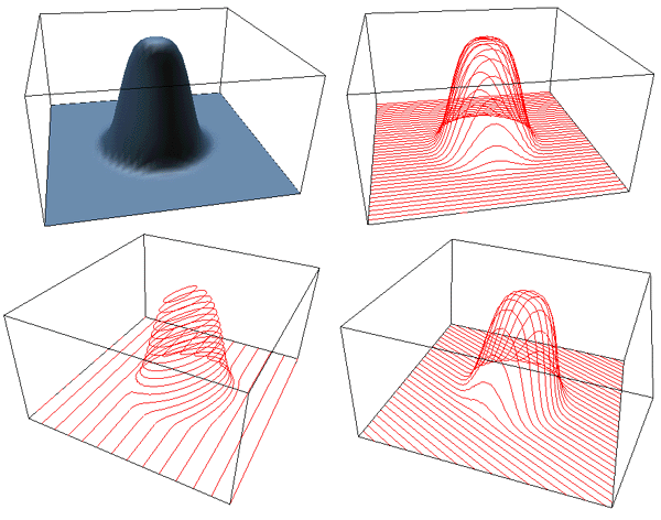
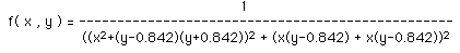
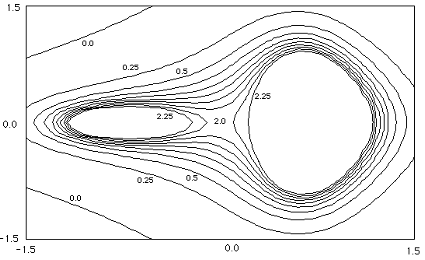
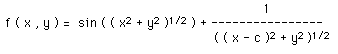
Example 1
Contour map and the following function
Example 2
Contour map and the following function
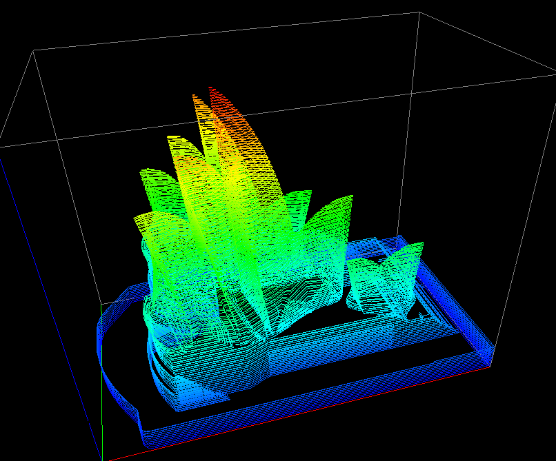
Example 3
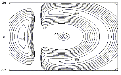
This is a more "real life" example where a C version of CONREC has been
used to contour a piece of landscape, the result is given below.
Images from the BYTE magazine version
Note
On occasion users have reported gaps in their contour lines, this should
of course never happen. There is however a pathological case that all
local contouring algorithms suffer from (local meaning that they only
use information in the immediate vicinity to determine the contour lines).
The problem arises when all four vertices of a grid cell have the
same value as the contour level under consideration. There are a number
of strategies that can be employed to overcome this special event,
the correct way is to consider a larger region in order to join up the
contours on either side of the problem cell. CONREC doesn't do this
and just leaves the cell without any contour lines thus resulting in
a gap. This special case essentially never happens for real values data,
it is most commonly associated with integer height datasets. The simplest
solution is to offset the contour levels being drawn by a very small amount.
|